Bottlenecks in LAMMPS
Overview
Teaching: 40 min
Exercises: 45 minQuestions
How can I identify the main bottlenecks in LAMMPS?
How do I come up with a strategy for finding the best optimisation?
What is load balancing?
Objectives
Learn how to analyse timing data in LAMMPS and determine bottlenecks
Earlier, you have learnt the basic philosophies behind various parallel computing methods (like MPI, OpenMP and CUDA). LAMMPS is a massively-parallel molecular dynamics package that is primarily designed with MPI-based domain decomposition as its main parallelization strategy. It supports all of the other parallelization techniques through the use of appropriate accelerator packages on the top of the intrinsic MPI-based parallelization.
So, is the only thing that needs to be done is decide on which accelerator package to use? Before using any accelerator package to speedup your runs, it is always wise to identify performance bottlenecks. The term “bottleneck” refers to specific parts of an application that are unable to keep pace with the rest of the calculation, thus slowing overall performance.
Therefore, you need to ask yourself these questions:
- Are my runs slower than expected?
- What is it that is hindering us getting the expected scaling behaviour?
Identify bottlenecks
Identifying (and addressing) performance bottlenecks is important as this could save you a lot of computation time and resources. The best way to do this is to start with a reasonably representative system having a modest system size and run for a few hundred/thousand timesteps.
LAMMPS provides a timing breakdown table printed at the end of log file and also within the screen output file generated at the end of each LAMMPS run. The timing breakdown table has already been introduced in the previous episode but let’s take a look at it again:
MPI task timing breakdown:
Section |  min time  |  avg time  |  max time  |%varavg| %total
---------------------------------------------------------------
Pair    | 1.5244     | 1.5244     | 1.5244     |   0.0 | 86.34
Neigh   | 0.19543    | 0.19543    | 0.19543    |   0.0 | 11.07
Comm    | 0.016556   | 0.016556   | 0.016556   |   0.0 |  0.94
Output  | 7.2241e-05 | 7.2241e-05 | 7.2241e-05 |   0.0 |  0.00
Modify  | 0.023852   | 0.023852   | 0.023852   |   0.0 |  1.35
Other   |            | 0.005199   |            |       |  0.29
Note that %total of the timing is giving for a range of different parts of the
calculation. In the following section, we will work on a few examples and try to
understand how to identify bottlenecks from this output. Ultimately, we will try to find
a way to minimise the walltime by adjusting the balance between
Pair, Neigh, Comm and the other parts of the calculation.
To get a feeling for this process, let us start with a Lennard-Jones (LJ) system. We’ll study two systems: the first one is with 4,000 atoms only; and the other one would be quite large, almost 10 million atoms. The following input file is for a LJ-system with an fcc lattice:
# 3d Lennard-Jones melt
variable        x index 10
variable        y index 10
variable        z index 10
variable        t index 1000

variable        xx equal 1*$x
variable        yy equal 1*$y
variable        zz equal 1*$z

variable        interval equal $t/2

units           lj
atom_style      atomic

lattice         fcc 0.8442
region          box block 0 ${xx} 0 ${yy} 0 ${zz}
create_box      1 box
create_atoms    1 box
mass            1 1.0

velocity        all create 1.44 87287 loop geom

pair_style      lj/cut 2.5
pair_coeff      1 1 1.0 1.0 2.5

neighbor        0.3 bin
neigh_modify    delay 0 every 20 check no

fix             1 all nve

thermo ${interval}
thermo_style custom step time  temp press pe ke etotal density
run             $t
We can vary the system size (i.e. number of atoms) by assigning appropriate
values to the variables x, y, and z at the beginning of the input file.
The length of the run can be decided by the
variable t. We’ll choose two different system sizes here: the one given is tiny just
having 4000 atoms (x = y = z = 10, t = 1000). If we take this input and modify it
such that x = y = z = 140 the other one would be huge
containing about 10 million atoms.
Important!
For many of these exercises, the exact modifications to job scripts that you will need to implement are system specific. Check with your instructor or your HPC institution’s helpdesk for information specific to your HPC system.
Also remember that after each execution the
log.lammpsfile in the current directory may be overwritten but you will still have the information we require in thempi-out.XXXXXfile corresponding to the executed job.
Example timing breakdown for 4000 atoms LJ-system
Using your previous job script for a a serial run (i.e. on a single core), replace the input file with the one for the small system (having 4000 atoms) and run it on the HPC system.
Take a look at the resulting timing breakdown table and discuss with your neighbour what you think you should target to get a performance gain.
Solution
Let us have a look at an example of the timing breakdown table.
MPI task timing breakdown:
Section |  min time  |  avg time  |  max time  |%varavg| %total
---------------------------------------------------------------
Pair    | 12.224     | 12.224     | 12.224     |   0.0 | 84.23
Neigh   | 1.8541     | 1.8541     | 1.8541     |   0.0 | 12.78
Comm    | 0.18617    | 0.18617    | 0.18617    |   0.0 |  1.28
Output  | 7.4148e-05 | 7.4148e-05 | 7.4148e-05 |   0.0 |  0.00
Modify  | 0.20477    | 0.20477    | 0.20477    |   0.0 |  1.41
Other   |            | 0.04296    |            |       |  0.30
The last
%totalcolumn in the table tells about the percentage of the total loop time is spent in this category. Note that most of the CPU time is spent onPairpart (~84%), about ~13% on theNeighpart and the rest of the things have taken only 3% of the total simulation time. So, in order to get a performance gain, the common choice would be to find a way to reduce the time taken by thePairpart since improvements there will have the greatest impact on the overall time. Often OpenMP or using a GPU can help us to achieve this…but not always! It very much depends on the system that you are studying (the pair styles you use in your calculation need to be supported).Serial timing breakdown for 10 million atoms LJ-system
The following table shows an example timing breakdown for a serial run of the large, 10 million atom system. Note that, though the absolute time to complete the simulation has increased significantly (it now takes about 1.5 hours), the distribution of
%totalremains roughly the same.MPI task timing breakdown: Section | min time | avg time | max time |%varavg| %total --------------------------------------------------------------- Pair | 7070.1 | 7070.1 | 7070.1 | 0.0 | 85.68 Neigh | 930.54 | 930.54 | 930.54 | 0.0 | 11.28 Comm | 37.656 | 37.656 | 37.656 | 0.0 | 0.46 Output | 0.1237 | 0.1237 | 0.1237 | 0.0 | 0.00 Modify | 168.98 | 168.98 | 168.98 | 0.0 | 2.05 Other | | 43.95 | | | 0.53
Effects due to system size on resource used
Different sized systems might behave differently as we increase our resource usage since they will have different distributions of work among our available resources.
Analysing the small system
Below is an example timing breakdown for 4000 atoms LJ-system with 40 MPI ranks
MPI task timing breakdown:
Section |  min time  |  avg time  |  max time  |%varavg| %total
---------------------------------------------------------------
Pair    | 0.24445    | 0.25868    | 0.27154    |   1.2 | 52.44
Neigh   | 0.045376   | 0.046512   | 0.048671   |   0.3 |  9.43
Comm    | 0.16342    | 0.17854    | 0.19398    |   1.6 | 36.20
Output  | 0.0001415  | 0.00015538 | 0.00032134 |   0.0 |  0.03
Modify  | 0.0053594  | 0.0055818  | 0.0058588  |   0.1 |  1.13
Other   |            | 0.003803   |            |       |  0.77
Can you discuss any observations that you can make from the above table? What could be the rationale behind such a change of the
%totaldistribution among various categories?Solution
The first thing that we notice in this table is that when we use 40 MPI processes instead of 1 process, percentage contribution of the
Pairpart to the total looptime has come down to about ~52% from 84%, similarly for theNeighpart also the percentage contribution reduced considerably. The striking feature is that theCommis now taking considerable part of the total looptime. It has increased from ~1% to nearly 36%. But why?We have 4000 total atoms. When we run this with 1 core, this handles calculations (i.e. calculating pair terms, building neighbour list etc.) for all 4000 atoms. Now when you run this with 40 MPI processes, the particles will be distributed among these 40 cores “ideally” equally (if there is no load imbalance (see below)). These cores then do the calculations in parallel, sharing information when necessary. This leads to the speedup. But this comes at a cost of communication between these MPI processes. So, communication becomes a bottleneck for such systems where you have a small number of atoms to handle and many workers to do the job. This implies that you really don’t need to waste your resource for such a small system.
Analysing the large system
Now consider the following breakdown table for the 10 million atom system with 40 MPI-processes. You can see that in this case, the
Pairterm is still dominating the table. Discuss about the rationale behind this.MPI task timing breakdown: Section | min time | avg time | max time |%varavg| %total --------------------------------------------------------------- Pair | 989.3 | 1039.3 | 1056.7 | 55.6 | 79.56 Neigh | 124.72 | 127.75 | 131.11 | 10.4 | 9.78 Comm | 47.511 | 67.997 | 126.7 | 243.1 | 5.21 Output | 0.0059468 | 0.015483 | 0.02799 | 6.9 | 0.00 Modify | 52.619 | 59.173 | 61.577 | 25.0 | 4.53 Other | | 12.03 | | | 0.92Solution
In this case, the system size is enormous. Each core will have enough atoms to deal with so it remains busy in computing and the time taken for the communication is still much smaller as compared to the “real” calculation time. In such cases, using many cores is actually beneficial.
One more thing to note here is the second last column
%varavg. This is the percentage by which the max or min varies from the average value. A value near to zero implies perfect load balance, while a large value indicated load imbalance. So, in this case, there is a considerable amount of load imbalance specially for theCommandPairpart. To improve the performance, one may like to explore a way to minimize load imbalance (but unfortunately we won’t have time to cover this topic).
Scalability
Since we have information about the timings for different components of the calculation, we can perform a scalability study for each of the components.
Investigating scalability on a number of nodes
Make a copy of the example input modified to run the large system (
x = y = z = 140).Now run the two systems using all the cores available in a single node and then run with more nodes (2, 4) with full capacity and note how this timing breakdown varies rapidly. While running with multiple cores, we’re using only MPI only as parallelization method.
You can use the job scripts from the previous episode as a starting point.
Using the
log.lammps(ormpi-out.XXXXX) files, write down the speedup factor for thePair,Commandwalltimefields in the timing breakdowns. Use the below formula to calculate speedup.(Speedup factor) = 1.0 / ( (Time taken by N nodes) / (Time taken by 1 node) )Note here how we have uses a node for our baseline unit of measurement (rather than a single processor) since running the serial case would take too long.
Using a simple pen and paper, make a plot of the speedup factor on the y-axis and number of processors on the x-axis for each of these fields.
What are your observations about this plot? Which fields show a good speedup factor? Discuss what could be a good approach in fixing this.
Solution
You should have noticed that
Pairshows almost perfect linear scaling, whereasCommshows poor scalability. and the total walltime also suffers from the poor scalability when running with more number of cores.However, remember this is a pretty small sample size, to do a definitive study more nodes/cores would need to be utilised.
MPI vs OpenMP
By now you should have developed some understanding on how can you use the timing breakdown table to identify performance bottlenecks in a LAMMPS run. But identifying the bottleneck is not enough, you need to decide what strategy would ‘probably’ be more sensible to apply in order to unblock the bottlenecks. The usual method of speeding up a calculation is to employ some form of parallelization. We have already discussed in a previous episode that there are many ways to implement parallelism in a code.
MPI based parallelism using domain decomposition lies at the core of LAMMPS. Atoms in each domain are associated to 1 MPI task. This domain decomposition approach comes with a cost however, keeping track and coordinating things among these domains requires communication overhead. It could lead to significant drop in performance if you have limited communication bandwidth, a slow network, or if you wish to scale to a very large number of cores.
While MPI offers domain based parallelization, one can also use parallelization over particles. This can, for example, be done using OpenMP which is a different parallelization paradigm based on threading. Moreover, OpenMP parallelization is orthogonal to MPI parallelization which means you can use them together. OpenMP also comes with an overhead: starting and stopping OpenMP takes compute time; OpenMP also needs to be careful about how it handles memory, the particular use case also impacts the efficiency. Remember that, in general, a threaded parallelization method in LAMMPS may not be as efficient as MPI unless you have situations where domain decomposition is no longer efficient (we will see below how to recognise such situations).
Let us discuss a few situations:
- The LJ-system with 4000 atoms (discussed above): Communication bandwidth with more
MPI processes. When you have too few atoms per domain, at some point LAMMPS will
not scale, and may even run slower, if you use more processors via
MPI only. With a pair style like
lj/cutthis will happen at a rather small number of atoms. - The LJ-system with with 10M atoms (discussed above): More atoms per processor, still communication is not a big deal in this case. This happens because you have a dense, homogeneous, well behaved system with a sufficient number of atoms, so that the MPI parallelization can be at its most efficient.
- Inhomogeneous or slab systems: In systems where there could be lots of empty spaces
in the simulation cell, the number of atoms handled across these domains will vary
a lot resulting in severe load balancing issue. While some of the domains will be
over-subscribed, some of them will remain under-subscribed causing these domains
(cores) to be less efficient in terms of performance. Often this could be improved by
using the
processorkeyword in a smart fashion, beyond that, there are the load balancing commands (balancecommand) and changing the communication using recursive bisecting and decomposition strategy. This might not help always since some of the systems are pathological. In such cases, a combination of MPI and OpenMP could often provide better parallel efficiency as this will result in larger subdomains for the same number of total processors and if you parallelize over particles using OpenMP threads, generally it does not hamper load balancing in a significant way. So, a sensible mix of MPI, OpenMP and thebalancecommand can help you to fetch better performance from the same hardware. - MD problems: For these, we need to deal with the calculation of electrostatic
interactions. Unlike the pair forces, electrostatic interactions are long range by
nature. To compute this long range interactions, very popular methods in MD are
ewaldandpppm. These long range solvers perform their computations in K-space. In case ofpppm, extra overhead results from the 3d-FFT, where as the Ewald method suffers from the poor \(O(N^\frac{3}{2})\) scaling, which will drag down the overall performance when you use more cores to do your calculation, even though Pair exhibits linear scaling. This is also a potential case where a hybrid run comprising of MPI and OpenMP might give you better performance and improve the scaling.
Let us now build some hands-on experience to develop some feeling on how this works.
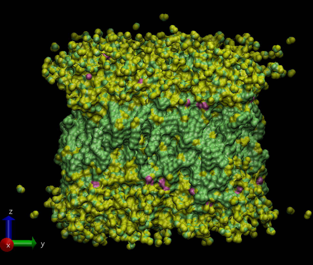
Case study: Rhodopsin system
The following input file,
in.rhodo, is one of the inputs provided in the bench directory of the LAMMPS distribution (version7Aug2019):# Rhodopsin model variable x index 1 variable y index 1 variable z index 1 variable t index 2000 units real neigh_modify delay 5 every 1 atom_style full # atom_modify map hash bond_style harmonic angle_style charmm dihedral_style charmm improper_style harmonic pair_style lj/charmm/coul/long 8.0 10.0 pair_modify mix arithmetic kspace_style pppm 1e-4 read_data data.rhodo replicate $x $y $z fix 1 all shake 0.0001 5 0 m 1.0 a 232 fix 2 all npt temp 300.0 300.0 100.0 & z 0.0 0.0 1000.0 mtk no pchain 0 tchain 1 special_bonds charmm thermo 500 thermo_style multi timestep 2.0 run $tNote that this input file requires an additional data file
data.rhodo.Using this you can perform a simulation of an all-atom rhodopsin protein in solvated lipid bilayer with CHARMM force field, long-range Coulombics interaction via PPPM (particle-particle particle mesh) and SHAKE constraints. The box contains counter-ions and a reduced amount of water to make a 32000 atom system. The force cutoff for LJ force-field is 10.0 Angstroms, neighbor skin cutoff is 1.0 sigma, number of neighbors per atom is 440. NPT time integration is performed for 20,000 timesteps.
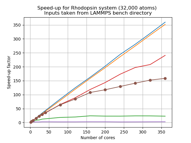
Let’s look at a scalability study of this system,
This was carried out on an Intel Skylake processor which has 2 sockets and 20 cores each, meaning 40 physical cores per node. Here jobs were run with 1, 4, 8, 16, 32, 40 processors, and then scaled up to 80, 120, 160, 200, 240, 280, 320, 360, 400 cores.
As we can see, similar to your own study,
PairandBondshow almost perfect linear scaling, whereasKspaceandCommshow poor scalability, and the total walltime also suffers from the poor scalability when running with more number of cores. This resembles situation 4 discussed above. A mix of MPI and OpenMP could be a sensible approach.
Load balancing
One important issue with MPI-based parallelization is that it can under-perform for systems with inhomogeneous distribution of particles, or systems having lots of empty space in them. It is pretty common that the evolution of simulated systems evolve over time to reflect such a case. This results in load imbalance. While some of the processors are assigned with finite number of particles to deal with for such systems, a few processors could have far less atoms (or none) to do any calculation and this results in an overall loss in parallel efficiency. This situation is more likely to expose itself as you scale up to a large large number of processors.
Let us take a look at another example from the LAMMPS bench directory with the input file
below which is run with
1 core (i.e., in serial) with x = y = z = 1, and t = 10,000.
variable        x index 1
variable        y index 1
variable        z index 1
variable        t index 10000

units           lj
atom_style      bond
atom_modify     map hash
special_bonds   fene

read_data       data.chain

replicate       $x $y $z

neighbor        0.4 bin
neigh_modify    every 1 delay 1

bond_style      fene
bond_coeff      1 30.0 1.5 1.0 1.0

pair_style      lj/cut 1.12
pair_modify     shift yes
pair_coeff      1 1 1.0 1.0 1.12

fix             1 all nve
fix             2 all langevin 1.0 1.0 10.0 904297

thermo          10000
timestep        0.012

run             $t
Example timing breakdown for system with low average number of neighbours
Section |  min time  |  avg time  |  max time  |%varavg| %total
---------------------------------------------------------------
Pair    | 20.665     | 20.665     | 20.665     |   0.0 | 18.24
Bond    | 6.9126     | 6.9126     | 6.9126     |   0.0 |  6.10
Neigh   | 57.247     | 57.247     | 57.247     |   0.0 | 50.54
Comm    | 4.3267     | 4.3267     | 4.3267     |   0.0 |  3.82
Output  | 0.000103   | 0.000103   | 0.000103   |   0.0 |  0.00
Modify  | 22.278     | 22.278     | 22.278     |   0.0 | 19.67
Other   |            | 1.838      |            |       |  1.62
Note that, in this case, the time spent in solving the
Pairpart is quite low as compared to theNeighpart. What do you think may have caused such an outcome?Solution
This kind of timing breakdown generally indicates either there is something wrong with the input or a very, very unusual system geometry. If you investigate the log file carefully, you would find that this is a system with a very short cutoff (1.12 sigma) resulting in on average less than 5 neighbors per atom (
Ave neighs/atom = 4.85891) and thus spending very little time on computing non-bonded forces.Being a sparse system, the necessity of rebuilding its neighbour lists is more frequent and this explains why the time spent of the
Neighpart is much more (about 50%) than thePairpart (~18%). On the contrary, the LJ-system is the extreme opposite. It is a relatively dense system having the average number of neighbours per atom nearly 37 (Ave neighs/atom = 37.4618). More computing operations are needed to decide the pair forces per atom (~84%), and less frequent would be the need to rebuild the neighbour list (~10%). So, here your system geometry is the bottleneck that causes the neighbour list building to happen too frequently and taking a significant part of the entire simulation time.
You can deal with load imbalance up to a certain extent using processors and balance
commands in LAMMPS. Detailed usage is given in the
LAMMPS manual. Unfortunately load balancing
is out of scope for this lesson since it is a somewhat complicated topic.
Key Points
The best way to identify bottlenecks is to run different benchmarks on a smaller system and compare it to a representative system
Effective load balancing is being able to distribute an equal amount of work across processes