Accelerating LAMMPS
Overview
Teaching: 30 min
Exercises: 90 minQuestions
What are the various options to accelerate LAMMPS?
What accelerator packages are compatible with which hardware?
How do I invoke a package in a LAMMPS run?
Objectives
Understand the different accelerator packages available in LAMMPS
Learn how to invoke the different accelerator packages across different hardwares
How can I accelerate LAMMPS performance?
There are two basic approaches to speed LAMMPS up. One is to use better algorithms for certain types of calculation, and the other is to use highly optimized codes via various “accelerator packages” for hardware specific platforms.
One popular example of the first approach is to use the Wolf summation method instead of the Ewald summation method for calculating long range Coulomb interactions effectively using a short-range potential. Similarly there are a few FFT schemes offered by LAMMPS and a user has to make a trade-off between accuracy and performance depending on their computational needs. This lesson is not aimed to discuss such types of algorithm-based speed-up of LAMMPS, instead we’ll focus on a few accelerator packages that are used to extract the most out of the available hardware of an HPC system.
There are five accelerator packages currently offered by LAMMPS. These are;
- OPT
- USER-INTEL
- USER-OMP
- GPU
- KOKKOS
Specialized codes contained in these packages help LAMMPS to perform well on the spectrum of architectures found in modern HPC platforms. Therefore, the next question that arises is: What hardware is supported by these packages?
Supported hardware
Here are some examples of the which packages support certain hardware:
Hardware Accelerator packages Multi-core CPUs OPT, USER-INTEL, USER-OMP, KOKKOS Intel Xeon Phi USER-INTEL, KOKKOS NVIDIA GPU GPU, KOKKOS
Within the limited scope of this tutorial, it is almost impossible to discuss all of the above packages in detail. The key point to understand is that, in all cases, the acceleration packages use multi-threading for parallelization, but how they do it and what architecture they can address differ.
The ONLY accelerator package that supports all kinds of hardware is KOKKOS. KOKKOS is a templated C++ library developed in Sandia National Laboratory and this helps to create an abstraction that allows a single implementation of a software application on different kinds of hardware. This will be discussed in detail in the next lesson.
In the meantime, we’ll touch a few key points about other accelerator packages to give you a feel about what these packages offer. To do this we will learn:
- how to invoke an accelerator package in a LAMMPS run
- how to gather data to compare the speedup with other LAMMPS runs.
Accelerator package overview
Precision
For many the accelerator packages you have the option to use
single,doubleormixedprecision. Precision means the amount of bytes that are used to store a number on a computer: the more bytes you use, the more precise the representation of a number you can have.doubleprecision uses double the amount of bytes assingleprecision. You should only use the precision that you need to, as higher precision comes with costs (more bytes for numbers means more work for the CPU, more storage and more bandwidth for communication).
mixedprecision is different in that it is implemented in an algorithm. It usually means you usesingleprecision when you can (to save CPU time and interconnect bandwidth) and double (or higher) precision when you have to (because you need numbers to a certain accuracy).
OPT package
- Only a handful of pair styles can be accelerated using this package (the list can be found here).
- Acceleration, in this case, is achieved by using a templated C++ library to reduce computational
overheads due to
iftests and other conditional code blocks.- This also provides better vectorization operations as compared to its regular CPU version.
- This generally offers 5-20% savings on computational cost on most machines
Effect on the timing breakdown table
We have discussed earlier that at the end of each run LAMMPS prints a timing breakdown table where it categorises the spent time into several categories (like
Pair,Bond,Kspace,Neigh,Comm,Output,Modify,Other). Can you make a justified guess about which of these category could be affected by the use of the OPT package?Solution
The
Paircomponent will see a reduction in cost since this accelerator package aims to work on the pair styles only.
USER-INTEL package
The USER-INTEL package supports single, double and mixed precision calculations.
Acceleration, in this case, is achieved in two different ways:
- Use vectorisation on multi-core CPUs
- Offload calculations of neighbour list and non-bonded interactions to Phi co-processors.
There are, however, a number of conditions:
- For using the offload feature, the (now outdated) Intel Xeon Phi coprocessors are required.
- For using vectorization feature, Intel compiler with version 14.0.1.106 or versions 15.0.2.044 and higher is required on both multi-core CPUs and Phi systems.
There are many LAMMPS features that are supported by this accelerator package, the list can be found here.
Performance enhancement using this package depends on many considerations, such as the
hardware that is available to you, the various styles that you are using in the input,
the size of your problem, and the selected precision. For example, if you are using a
pair style (say, reax) for which this is not implemented, its obvious that you are not
going to have a performance gain for the Pair part of the calculation. If the
majority of the computation time is coming from the Pair part then you are in trouble.
If you would like to know how much speedup you can expect to achieve using USER-INTEL, you can
take a look in the corresponding
LAMMPS documentation.
USER-OMP package
This accelerator package offers performance gain through optimisation and multi-threading via the OpenMP interface. In order to make the multi-threading functional, you will need multi-core CPUs and a compiler that supports multi-threading. If your compiler does not support multi-threading then also you can still use it as an optimized serial code.
A large sub-set of the LAMMPS routines can be used with this accelerator. A list of functionalities enabled with this package can be found here.
Generally, one can expect 5-20% performance boost when using this package even in serial! You should always test to figure out what the optimal number of OpenMP threads to use for a particular simulation is. Typically, the package gives better performance when used for lower numbers of threads, for example 2-4. It is important to remember that the MPI implementation in LAMMPS is so robust that you may almost always expect this to be more effective than using OpenMP on multi-core CPUs.
GPU package
Using the GPU package in LAMMPS, one can achieve performance gain by coupling GPUs to one or many CPUs. The package supports both CUDA (which is vendor specific) and OpenCL (which is an open standard) so it can be used on a variety of GPU hardware.
Calculations that require access to atomic data like coordinates, velocities, forces may suffer bottlenecks since at every step these data are communicated back and forth between the CPUs and GPUs. Calculations can be done in single, double or mixed precisions.
In case of the GPU package, computations are shared between CPUs and GPUs (unlike the KOKKOS package GPU implementation where the primary aim is to offload all of the calculations to the GPUs only). For example, asynchronous force calculations like pair vs bond/angle/dihedral/improper can be done simultaneously on GPUs and CPUs respectively. Similarly, for PPPM calculations the charge assignment and the force computations are done on GPUs whereas the FFT calculations that require MPI communications are done on CPUs. Neighbour lists can be built on either CPUs or GPUs. You can control this using specific flags in the command line of your job submission script. Thus the GPU package can provide a balanced mix of GPU and CPU usage for a particular simulation to achieve a performance gain.
A list of functionalities enabled with this package can be found here.
KOKKOS package
The KOKKOS package in LAMMPS is implemented to gain performance with portability. This will be discussed in more depth in the next lesson.
How to invoke a package in LAMMPS run?
Let us now come back to the Rhodopsin example for which we showed a thorough scaling
study in the previous episode.
We found that the Kspace and Neigh calculations
suffer from poor scalability as you increase number of cores to do the calculations. In
such situation a hybrid approach combining parallelizing over domains (i.e. MPI-based)
and parallelizing over atoms (i.e. thread-based OpenMP) could be more beneficial to
improve scalability than a pure MPI-based approach. To test this, in the following
exercise, we’ll do a set of calculations to mix MPI and OpenMP using the USER-OMP
package. Additionally, this exercise will also help us to learn the basic principles of
invoking accelerator packages in a LAMMPS run.
To call an
accelerator package (USER-INTEL, USER-OMP, GPU, KOKKOS) in
your LAMMPS run, you need to know a LAMMPS command called package. This command
invokes package-specific settings for an accelerator. You can learn about this command
in detail from the
LAMMPS manual. Before starting our runs, let
us discuss the syntax of the package command in LAMMPS. The basic syntax for the
additional options to the LAMMPS are:
package <style> <arguments>
<style> allows you to choose the accelerator package for your run. There are four different
packages available currently (version 3Mar20):
intel: This calls the USER-INTEL packageomp: This calls the USER-OMP packagegpu: This calls the GPU packagekokkos: This calls the KOKKOS package
<arguments> are then the list of arguments you wish to provide to your <style> package.
How to invoke the USER-OMP package
To call USER-OMP in a LAMMPS run, use omp as <style>. Next you need to choose
proper <arguments> for the omp style. The minimum content of <arguments> is the number
of OpenMP threads that you like to associate with each MPI process. This is an integer
and should be chosen sensibly. If you have N number of physical cores available per node
then;
(Number of MPI processes) x (Number of OpenMP threads) = (Number of cores per node)
<arguments> can potentially include an additional number of keywords and their
corresponding values.
These keyword/values provides with you enhanced flexibility to distribute your job among
the MPI ranks and threads. For a quick reference, the following table could be useful:
| Keyword | values | What it does? |
|---|---|---|
neigh |
yes |
threaded neighbor list build (this is the default) |
neigh |
no |
non-threaded neighbor list build |
There are two alternate ways to add these options to your simulation:
-
Edit the input file and introduce the line describing the
packagecommand in it. This is perfectly fine, but always remember to use this near the top of the script, before the simulation box has been defined. This is because it specifies settings that the accelerator packages use in their initialization, before a simulation is defined.An example of calling the USER-OMP package for a LAMMPS input file is given below:
package omp 4 neigh no(here 4 is the number of OpenMP threads per MPI task)
To distinguish the various styles of these accelerator packages from its ‘regular’ non-accelerated variants, LAMMPS has introduced suffixes for styles that map to
packagenames. When using input files, you also need to append an extra/ompsuffix wherever applicable to indicate the accelerator package is used for a style. For example, if we take a pair potential that would normally be set withlj/charmm/coul/long, when using USER-OMP optimization it would be set in the input file as:pair_style lj/charmm/coul/long/omp 8.0 10.0 -
A simpler way to do this is through the command-line when launching LAMMPS using the
-pkcommand-line switch. The syntax would be essentially the same as when used in an input script:srun lmp -in in.lj -sf omp -pk omp $OMP_NUM_THREADS neigh nowhere
OMP_NUM_THREADSis now an environment variable that we can use to control the number of OpenMP threads. This second method appears to be convenient since you don’t need to edit the input file (and possibly in many places)!Note that there is an extra command-line switch in the above command-line. Can you imagine this is for? The
-sfswitch auto-appends the provided accelerator suffix to various styles in the input script. Therefore, when an accelerator package is invoked through the-pkswitch (for example,-pk ompor-pk gpu), the-sfswitch ensures that the appropriate style is also being invoked in the simulation (for example, it ensures that thelj/cut/gpuis used instead oflj/cutaspair_style, or,lj/charmm/coul/long/ompis used in place oflj/charmm/coul/long).
In this tutorial, we’ll stick to the second method of invoking the accelerator package, i.e. through the command-line.
Case study: Rhodopsin (with USER-OMP package)
We shall use the same input file for the rhodopsin system with lipid bilayer that was described in the case study of our previous episode. In this episode, we’ll run this using the USER-OMP package to mix MPI and OpenMP. For all the runs we will use the default value for the
neighkeyword (which means we can exclude it from the command line).
First, find out the number of cpu cores available per node in the HPC system that you are using and then figure out all the possible MPI/OpenMP combinations that you can have per node. For example on a node with 40 physical cores, there are 8 combinations per node. Write down the different combinations for your machine.
Here we have a job script to run the rhodopsin case with 2 OpenMP threads per MPI task, choose another MPI/OpenMP combination and adapt (and run) the job script:
#!/bin/bash -x

# Ask for 1 nodes of resources for an MPI/OpenMP job for 5 minutes

#SBATCH --account=ecam
#SBATCH --nodes=1
#SBATCH --output=mpi-out.%j
#SBATCH --error=mpi-err.%j
#SBATCH --time=00:10:00

# Let's use the devel partition for faster queueing time since we have a tiny job.
# (For a more substantial job we should use --partition=batch)

#SBATCH --partition=devel

# Make sure that the multiplying the following 2 gives ncpus per node (24)

#SBATCH --ntasks-per-node=12
#SBATCH --cpus-per-task=2

# Prepare the execution environment
module purge
module use /usr/local/software/jureca/OtherStages
module load Stages/Devel-2019a
module load intel-para/2019a
module load LAMMPS/3Mar2020-Python-3.6.8-kokkos

# Also need to export the number of OpenMP threads so the application knows about it
export OMP_NUM_THREADS=$SLURM_CPUS_PER_TASK

# srun handles the MPI placement based on the choices in the job script file
srun lmp -in in.rhodo -sf omp -pk omp $OMP_NUM_THREADS
On a system of a node with 40 cores, if we want to see scaling, say up to 10 nodes, this means that a total of 80 calculations would need to be run since we have 8 MPI/OpenMP combinations for each node.
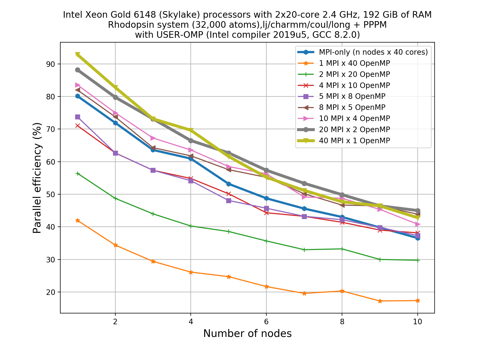
Thankfully, you don’t need to do the 80 calculations right now! Here’s an example plot for what that picture might look like:
Write down your observations based on this plot and make comments on any performance enhancement when you compare these results with the pure MPI runs.
Solution
For a system with 40 cores per node, the following combinations are possible:
- 1 MPI task with 40 OpenMP threads
- 2 MPI tasks with 20 OpenMP threads
- 4 MPI tasks with 10 OpenMP threads
- 5 MPI tasks with 8 OpenMP threads
- 8 MPI tasks with 5 OpenMP threads
- 10 MPI tasks with 4 OpenMP threads
- 20 MPI tasks with 2 OpenMP threads
- 40 MPI tasks with 1 OpenMP threads
For a perfectly scalable system, parallel efficiency should be equal to 100%, and as it approaches zero we say that the parallel performance is poor.
From the plot, we can make a few observations.
- As we increase number of nodes, the parallel efficiency decreases considerably for all the runs. This decrease in performance could be associated to the poor scalability of the
KspaceandNeighcomputations.- Parallel efficiency is increased by about 10-15% when we use mixed MPI+OpenMP approach even when we use only 1 OpenMP thread.
- The performance of hybrid runs are better than or comparable to pure MPI runs only when the number of OpenMP threads are less than or equals to five. This implies that USER-OMP package shows scalability only with lower numbers of threads.
Though we are seeing about 10-15% increase in parallel efficiency of hybrid MPI+OpenMP runs (using 2 threads) over pure MPI runs, still it is important to note that trends in loss of performance with increasing core number is similar in both of these types of runs thus indicating that this increase in performance might not be due to threading but rather due to other effects (like vectorisation).
In fact, there are overheads to making the kernels thread-safe. In LAMMPS, MPI-based parallelization almost always win over OpenMP until thousands of MPI ranks are being used where communication overheads become very significant.
How to invoke the GPU package
A question that you may be asking is how much speed-up would you expect from the GPU package. Unfortunately there is no easy answer for this. This can depend on many things starting from the hardware specification to the complexities involved with the specific problem that you are simulating. However, for a given problem one can always optimize the run-time parameters to extract the most out of a hardware. In the following section, we’ll discuss some of these tuning parameters for the simplest LJ-systems.
The primary aim for this following exercise is:
- To get a basic understanding of the various command line arguments that can control how a job is distributed among CPUs/GPUs, how to control CPU/GPU communications, etc.
- To get an initial idea on how to play with different run-time parameters to get an optimum performance.
- Finally, one can also make a fair comparison of performance between a regular LAMMPS run, the GPU package and a KOKKOS implementation of GPU functionality.
- Moreover, this exercise will also help the users to extend the knowledge of using the package command so that they can figure out by themselves how to use other accelerator packages in LAMMPS.
Before invoking the GPU package, you must ask the following questions:
- Do I have an access to a computing node with a GPU?
- Is my LAMMPS binary built with GPU package? HOW TO CHECK THIS?
If the answer to these two questions is a yes then we you can proceed to the following section.
Basic syntax: arguments and keywords
As discussed above, you need to use the package command to invoke the GPU package.
To use the GPU package for an accelerator you need to select gpu as <style>. Next
you need to choose proper <arguments> for the gpu style. The main argument for the
gpu style is:
ngpu: This sets the number of GPUs per node. There must be at least as many MPI tasks per node as GPUs. If there are more MPI tasks (per node) than GPUs, multiple MPI tasks will share each GPU (which may not be optimal).
In <arguments>, we can also have a number of keywords and their corresponding
values. These keyword/values provides you enhanced flexibility to distribute your
job among CPUs and GPUs in an optimum way. For a quick reference, the table below
could be useful.
Keywords of the GPU package
For more details, see the official documentation for LAMMPS.
Keywords Use Default value neighspecifies where neighbor lists for pair style computation will be built: GPU or CPU. yesnewtonsets the Newton flags for pairwise (not bonded) interactions to off or on. Only off value is supported with the GPU package currently (version 3Mar20)off(only)binsizesets the size of bins used to bin atoms in neighbor list builds performed on the GPU, if neigh = yes is set 0.0 splitused for load balancing force calculations between CPU and GPU cores in GPU-enabled pair styles 1.0(all on GPU),-1.0(dynamic load balancing), 0 <split<1.0 (custom)gpuIDallows selection of which GPUs on each node will be used for a simulation tpasets the number of GPU thread per atom used to perform force calculations. It is used for fining tuning of performance. When you use large cutoffs or do a simulation with a small number of particles per GPU, you may increase the value of this keyword to see if it can improve performance. The number of threads per atom must be chosen as a power of 2 and cannot be greater than 32 (version 3Mar20).1deviceused to tune parameters optimized for a specific accelerator and platform when using OpenCL blocksizeallows you to tweak the number of threads used per thread block minimum = 32
Not surprisingly, the syntax we use is similar to that of USER-OMP package:
srun lmp -in in.lj -sf gpu -pk gpu 2 neigh yes newton off split 1.0
Learn to call the GPU package from the command-line
Derive a command line to submit a LAMMPS job for the LJ system described by the following input file (
in.lj). Use command/package keywords from the table should to set the following conditions:
- Use 4 GPUs and a full node of MPI ranks
- Neighbour lists built on CPUs
- Dynamic load balancing between CPUs and GPUs
# 3d Lennard-Jones melt
variable        x index 60
variable        y index 60
variable        z index 60
variable        t index 500

variable        xx equal 1*$x
variable        yy equal 1*$y
variable        zz equal 1*$z

variable        interval equal $t/2

units           lj
atom_style      atomic

lattice         fcc 0.8442
region          box block 0 ${xx} 0 ${yy} 0 ${zz}
create_box      1 box
create_atoms    1 box
mass            1 1.0

velocity        all create 1.44 87287 loop geom

pair_style      lj/cut 2.5
pair_coeff      1 1 1.0 1.0 2.5

neighbor        0.3 bin
neigh_modify    delay 0 every 20 check no

fix             1 all nve

thermo          ${interval}
thermo_style custom step time  temp press pe ke etotal density
run             $t
Solution
srun lmp -in in.lj -sf gpu -pk gpu 2 neigh no newton off split -1.0The breakdown of the command is as follows;
-pk gpu 4- Setting GPU package and number of GPUs (2)-sf gpu- GPU package related fix/pair stylesneigh no- Anovalue ofneighkeyword indicates neighbour list built in the CPUsnewton off- Currently, only an off value is allowed as all GPU package pair styles require this setting.split -1.0- Dynamic load balancing option between CPUs and GPUs when value =-1NB: It is important to fix the number of MPI ranks in your submission script, and request the number of GPUs you wish to utilise. These will change depending on your system.
How to request and configure GPU resources is usually quite specific to the HPC system you have access to. Below you will find an example of how to submit the job we just constructed to JURECA.
#!/bin/bash -x

# Ask for 1 nodes of resources for an MPI/GPU job for 10 minutes

#SBATCH --account=ecam
#SBATCH --nodes=1
#SBATCH --output=mpi-out.%j
#SBATCH --error=mpi-err.%j
#SBATCH --time=00:10:00

# Configure the GPU usage (we request to use all 4 GPUs on a node)
#SBATCH --partition=develgpus
#SBATCH --gres=gpu:4

# Use this many MPI tasks per node (maximum 24)
#SBATCH --ntasks-per-node=24

module purge
module use /usr/local/software/jureca/OtherStages
module load Stages/Devel-2019a
module load intel-para/2019a
# Note we are loading a different LAMMPS package
module load LAMMPS/9Jan2020-cuda

srun lmp -in in.lj -sf gpu -pk gpu 4 neigh no newton off split -1.0
Understanding the GPU package output
At this stage, once you complete a job successfully, it is time to look for a few things in the LAMMPS output file. The first of these is to check that LAMMPS is doing the things that you asked for and the rest are to tell you about the performance outcome.
It prints about the device information both in the screen-output and the log file. You would notice something similar to;
-------------------------------------------------------------------------------
- Using acceleration for lj/cut:
-  with 12 proc(s) per device.
-  with 1 thread(s) per proc.
-------------------------------------------------------------------------------
Device 0: Tesla K80, 13 CUs, 10/11 GB, 0.82 GHZ (Double Precision)
Device 1: Tesla K80, 13 CUs, 0.82 GHZ (Double Precision)
-------------------------------------------------------------------------------

Initializing Device and compiling on process 0...Done.
Initializing Devices 0-1 on core 0...Done.
Initializing Devices 0-1 on core 1...Done.
Initializing Devices 0-1 on core 2...Done.
Initializing Devices 0-1 on core 3...Done.
Initializing Devices 0-1 on core 4...Done.
Initializing Devices 0-1 on core 5...Done.
Initializing Devices 0-1 on core 6...Done.
Initializing Devices 0-1 on core 7...Done.
Initializing Devices 0-1 on core 8...Done.
Initializing Devices 0-1 on core 9...Done.
Initializing Devices 0-1 on core 10...Done.
Initializing Devices 0-1 on core 11...Done.
The first thing that you should notice here is that it’s using an acceleration for the
pair potential lj/cut
and for this purpose it is using two devices (Device 0 and Device 1) and 12 MPI-processes per
device. That is what we asked for using 2 GPUs (-pk gpu 2) and in this case there
were 24 cores on the node. The number of tasks is shared equally by
each GPU. The detail about the graphics card is also printed, along
with the numerical precision used by the GPU package is also printed. In this case, it
is using double precision. Next it shows how many MPI-processes are spawned per GPU.
Accelerated version of pair-potential
This section of the output shows you that it is actually using the accelerated version of the
pair potential lj/cut. You can see that it is using lj/cut/gpu though in your input file you
mentioned this as pair_style lj/cut 2.5. This is what happens when you use the -sf gpu
command-line switch. This automatically ensures that the correct accelerated version is called for
this run.
(1) pair lj/cut/gpu, perpetual
    attributes: full, newton off
    pair build: full/bin/anomaly
    stencil: full/bin/3d
    bin: standard
Performance section
The following screen-output tells you all about the performance. Some of these terms are already
discussed in the previous episode.
When you use the
GPU package you see an extra block
of information known as Device Time Info (average). This gives you a breakdown of how
the devices (GPUs) have been utilised to do various parts of the job.
Loop time of 7.56141 on 24 procs for 500 steps with 864000 atoms

Performance: 28566.100 tau/day, 66.125 timesteps/s
95.3% CPU use with 24 MPI tasks x 1 OpenMP threads

MPI task timing breakdown:
Section |  min time  |  avg time  |  max time  |%varavg| %total
---------------------------------------------------------------
Pair    | 2.2045     | 2.3393     | 2.6251     |   6.1 | 30.94
Neigh   | 2.8258     | 2.8665     | 3.0548     |   2.9 | 37.91
Comm    | 1.6847     | 1.9257     | 2.0968     |   6.8 | 25.47
Output  | 0.0089157  | 0.028466   | 0.051726   |   6.7 |  0.38
Modify  | 0.26308    | 0.27673    | 0.29318    |   1.5 |  3.66
Other   |            | 0.1247     |            |       |  1.65

Nlocal:    36000 ave 36186 max 35815 min
Histogram: 1 2 3 4 2 3 3 4 1 1
Nghost:    21547.7 ave 21693 max 21370 min
Histogram: 1 1 0 5 5 2 4 1 2 3
Neighs:    0 ave 0 max 0 min
Histogram: 24 0 0 0 0 0 0 0 0 0
FullNghs:  2.69751e+06 ave 2.71766e+06 man 2.6776e+06 min
Histogram: 1 1 4 4 3 2 3 4 1 1

Total # of neighbors = 64740192
Ave neighs/atom = 74.9308
Neighbor list builds = 25
Dangerous builds not checked


---------------------------------------------------------------
      Device Time Info (average):
---------------------------------------------------------------
Data Transfer:   0.9243 s.
Data Cast/Pack:  0.6464 s.
Neighbor copy:   0.5009 s.
Neighbor unpack: 0.0000 s.
Force calc:      0.6509 s.
Device Overhead: 0.5445 s.
Average split:   0.9960.
Threads / atom:  4.
Max Mem / Proc:  53.12 MB.
CPU Driver_Time: 0.5243 s.
CPU Idle_Time:   0.9986 s.
---------------------------------------------------------------


Please see the log.cite file for references relevant to this simulation

Total wall time: 0:00:15
Choosing your parameters
You should now have an idea of how to submit a LAMMPS job that uses the GPU package as an accelerator. Optimizing the run may not be that straight-forward however. You can have numerous possibilities of choosing the argument and the keywords. Not only that, the host CPU might have multiple cores. More choices would arise from here.
As a rule of thumb, you must have at least same number of MPI processes as the number of GPUs available to you. But often, using many MPI tasks per GPU gives you the better performance. As an example, if you have 4 physical GPUs, you must initiate (at least) 4 MPI processes for this job. Let’s assume that you have a CPU with 12 cores. This gives you flexibility to use at most 12 MPI processes and the possible combinations are 4 GPUs with 4 CPUs, 4 GPUs with 8 CPUs and 4 GPUs with 12 CPUs. Though it may sound like that 4 GPUs with 12 CPUs will provide the maximum speed-up, that may not be the case! This entirely depends on the problem and also on other settings which can in general be controlled by the keywords mentioned in the above table. Moreover, one may find that for a particular problem using 2 GPUs instead of 4 GPUs may give better performance, and this is why it is advisable to figure out the best possible set of run-time parameters by following a thorough optimization before starting the production runs. This might save you a lot of resources and time!
Case study
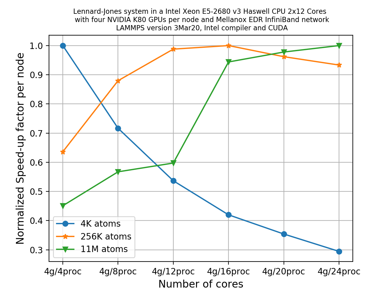
Let’s look at the result of doing such a study for a node with 4 GPUs and 24 CPU cores. We set
t = 5000and use 3 sets of values for our volume:
x = y = z = 10= 4,000 atomsx = y = z = 40= 256,000 atomsx = y = z = 140= 11,000,000 atomsWe choose package keywords such that neighbour list building and force computations are done entirely on the GPUs:
-sf gpu -pk gpu 4 neigh yes newton off split 1.0where 4 GPUs are being used.
On a system with 2x12 cores per node and four GPUs, the different combinations are;
- 4 GPUs/4 MPI tasks
- 4 GPUs/8 MPI tasks
- 4 GPUs/12 MPI tasks
- 4 GPUs/16 MPI tasks
- 4 GPUs/20 MPI tasks
- 4 GPUs/24 MPI tasks
Across all GPU/MPI combinations and system sizes (4K, 256K, 11M), there are a total of 18 runs. The final plot is shown below.
What observations can you make about this plot?
Solution
The main observations you can take from this are:
- For the system with 4000 atoms, increasing the number of MPI tasks actually degrades the overall performance.
- For the 256K system, we can notice an initial speed-up with increasing MPI task counts up to 4 MPI ranks per GPU, and then it starts declining again.
- For the largest 11M atom system, there is a sharp increase of speed-up up to 4 MPI ranks per GPU, and then also a relatively slow but steady increase is seen with increasing MPI tasks per GPU (in this case, 6 MPI tasks per GPU).
Possible explanation:
- For the smallest system, the number of atoms assigned to each GPU or MPI ranks is very low. The system size is so small that considering GPU acceleration is practically meaningless. In this case you are employing far too many workers to complete a small job and therefore it is not surprising that the scaling deteriorates with increasing MPI tasks. In fact, you may try to use 1 GPU and a few MPI task to see if the performance increases in this case.
- As the system size increases, the normalized speed-up factor per node increases with increasing MPI tasks per GPU since in these cases the MPI tasks are busy in computing rather than spending time in communicating each other, i.e. computational overhead exceeds the communication overheads.
Load balancing: revisited
We have discussed load balancing in the previous episode due to the potential for under-performance
in systems with an inhomogeneous distribution of particles. We discussed earlier that it can be
done using the split keyword. Using this keyword a fixed fraction of particles is offloaded to
the GPU while force calculation for the other particles occurs simultaneously on the CPU. When you
set split = 1 you are offloading entire force computations to the GPUs (discussed in previous
exercise). What fraction of particles would be offloaded to GPUs can be set explicitly by choosing
a value ranging from 0 to 1. When you set its value to -1, you are switching on dynamic load
balancing. This means that LAMMPS selects the split factor dynamically.
Switching on dynamic load balancing
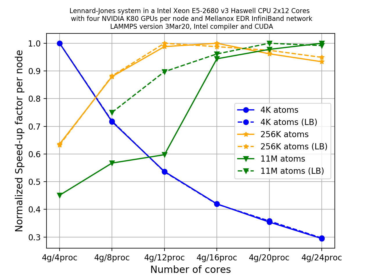
If we repeat the previous exercise but this time use dynamic load balancing (by changing the value of
splitto-1.0). We can see how the plot has changed significantly due to dynamic load balancing increasing the performance.
CPU versus GPU
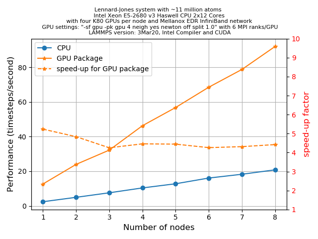
By now we have idea about some of the ‘preferred’ tuning parameters for an LJ-system. For the current exercise, let us take the system with ~11 million atoms, i.e.
x = y = z = 140andt = 500and for this size of atoms, we know from our previous example thatA GPUs/B MPItasks (whereAis number of GPUs andBis number of cores in a node) gives the best performance. We wish to see how much acceleration a GPU package can provide if we offload the entire force computation and neighbour list building to the GPUs. This can be done using;-sf gpu -pk gpu 4 neigh yes newton off split 1.0The plot below shows an HPC system with 2x12 CPU cores per node and 2 GPUs (4 visible devices) per node. Two sets of runs (i.e. with and without the GPU package) were executed with up to 8 nodes. Performance data was extracted from the log files in the unit of
timesteps/s, and speed-up factors were calculated for each node.
We can see a reasonable acceleration when we use the GPU package for all the runs consistently. The calculated speed-up factors show that we obtain maximum speed-up (~5.2x) when we use 1 node, then it gradually decreases (for 2 nodes it is 5x) and finally saturates to a value of ~4.25x when we run using 3 nodes or higher (up to 8 nodes is tested here).
The slight decrease in speed-up with increasing number of nodes could be related to the inter-node communications. But overall the GPU package offers quite a fair amount of performance enhancement over the regular CPU version of LAMMPS with MPI parallelization.
Key Points
The five accelerator packages currently offered by LAMMPS are i) OPT, ii) USER-INTEL, iii) USER-OMP, iv) GPU, v) KOKKOS
KOKKOS is available for use on all types of hardware. Other accelerator packages are hardware specific
To invoke a package in LAMMPS, the notation is
package <style> <arguments>, wherestyleis the package you want to invoke