Why bother with performance?
Overview
Teaching: 10 min
Exercises: 5 minQuestions
What is software performance?
Why is software performance important?
How can performance be measured?
What is meant by flops, walltime and CPU hours?
How can performance be enhanced?
How can I use compute resources effectively?
Objectives
Understand the link between software performance and hardware
Identify the different methods of enhancing performance
Calculate walltime, CPU hours
What is software performance?
Before getting into the software side of things, lets take a few steps back. The concept of performance is generic and can apply to many factors in our lives, such as our own physical and mental performance. With software performance the emphasis is not on using the most powerful machine, but on how best to utilise the power that you have.
Say you are the chef in a restaurant and every dish that you do is perfect. You would be able to produce a set 7 course meal for a table of 3-6 without too much difficulty. If you are catering a conference dinner though, it becomes more difficult, as people would be waiting many hours for their food. However, if you could delegate tasks to a team of 6 additional chefs who could assist you (while also communicating with each other), you have a much higher chance of getting the food out on time and coping with a large workload. With 7 courses and a total of 7 chefs, it’s most likely that each chef will spend most of their time concentrating on doing one course.
When we dramatically increase the workload we need to distribute it efficiently over the resources we have available so that we can get the desired result in a reasonable amount of time. That is the essence of software performance, using the resources you have to the best of their capabilities.
Why is software performance important?
This is potentially a complex question but has a pretty simple answer when we restrict ourselves to the context of this lesson. Since the focus here is our usage of software that is developed by someone else, we can take a self-centred and simplistic approach: all we care about is reducing the time to solution to an acceptable level while minimising our resource usage.
This lesson is about taking a well-informed, systematic approach towards how to do this.
Enhancing performance: rationale
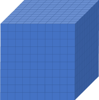
Imagine you had a
10x10x10box like the one below, divided up into smaller boxes, each measuring1x1x1. In one hour, one CPU core can simulate one hour of activity inside the smaller box. If you wanted to simulate what was happening inside the large box for 8 hours, how long will it take to run if we only use one CPU core?
Solution
8000 hours…close to a year!
This is way longer than is feasibly convenient! But remember, that is utilising just one core. If you had a machine that could simulate each of those smaller boxes simultaneously and a code that enables each box to effectively interact with each other, the whole job would only take roughly an hour (but probably a little more because of issues we will discuss in subsequent episodes).
How is performance measured?
There are a number of key terms in computing when it comes to understanding performance and expected duration of tasks. The most important of these are walltime, flops and CPU hours.
Walltime
Walltime is the length of time, usually measured in seconds, that a program takes to run (i.e., to execute its assigned tasks). It is not directly related to the resources used, it’s the time it takes according to an independent clock on the wall.
Flops
Flops (or sometimes flop/s) stands for floating point operations per second and they are typically used to measure the (theoretical) performance of a computer’s processor.
The theoretical peak flops is given by
Number of cores * Average frequency * Operations per cycle`What a software program can achieve in terms of flops is usually a surprisingly small percentage of this value (e.g., 10% efficiency is not a bad number!).
Since in our case we don’t develop or compile the code, the only influence we have on the flops achieved by the application is by dictating the choices it makes during execution (sometimes called telling it what code path to walk).
CPU Hours
CPU hours is the amount of CPU time spent processing. For example, if I execute for a walltime of 1 hour on 10 CPUs, then I will have used up 10 CPU hours.
Maximising the flops of our application will help reduce the CPU hours, since we will squeeze more calculations out of the same CPU time. However, you can achieve much greater influence on the CPU hours by using a better algorithm to get to your result. The best algorithm choice is usually heavily dependent on your particular use case (and you are always limited by what algorithm options are available in the software).
Calculate CPU hours
Assume that you are utilising all the available cores in a node with 40 CPU cores. Calculate the CPU hours you would need if you expect to run for 5 hours using 2 nodes.
How much walltime do you need?
How do you ask the resource scheduler for that much time?
Solution
400 CPU hours are needed.
We need to ask the scheduler for 5 hours (and 2 nodes worth of resources for that time). To ask for this from the scheduler we need to include the appropriate option in our job script:
#SBATCH -t 5:00:00
The -t option to the scheduler used in the exercise indicates the
maximum amount of walltime requested, which will differ from the actual
walltime the code spends to run.
How can we enhance performance?
If you are taking this course you are probably application users, not application developers. To enhance the code performance you need to trigger behaviour in the software that the developers will have put in place to potentially improve performance. To do that, you need to know what the triggers are and then try them out with your use case to see if they really do improve performance.
Some triggers will be hardware related, like the use of OpenMP, MPI, or GPUs. Others might relate to alternative libraries or algorithms that could be used by the application.
Enhancing Performance
Which of these are viable ways of enhancing performance? There may be more than one correct answer.
- Utilising more CPU cores and nodes
- Increasing the simulation walltime
- Reduce the frequency of file writing in the code
- Having a computer with higher flops
Solution
- Yes, potentially, the more cores and nodes you have, the more work can be distributed across those cores…but you need to ensure they are being used!
- No, increasing simulation walltime only increases the possible duration the code will run for. It does not improve the code performance.
- Yes, IO is a very common bottleneck in software, it can be very expensive (in terms of time) to write files. Reducing the frequency of file writing can have a surprisingly large impact.
Yes, in a lot of cases the faster the computer, the faster the code can run. However, you may not be able to find a computer with higher flops, since higher individual CPU flops need disproportionately more power to run (so are not well suited to an HPC system).
In an HPC system, you will usually find a lot of lower flop cores because they make sense in terms of the use of electrical energy. This surprises people because when they move to an HPC system, they may initially find that their code is slower rather than faster. However, this is usually not about the resources but managing their understanding and expectations of them.
As you can see, there are a lot of right answers, however some methods work better than others, and it can entirely depend on the problem you are trying to solve.
How can I use compute resources effectively?
Unfortunately there is no simple answer to this, because the art of getting the ‘optimum’ performance is ambiguous. There is no ‘one size fits all’ method to performance optimization.
While preparing for production use of software, it is considered good practice to test performance on manageable portion of your problem first, attempt to optimize it (using some of the recommendations we outline in this lesson, for example) and then make a decision about how to run things in production.
Key Points
Software performance is the use of computational resources effectively to reduce runtime
Understanding performance is the best way of utilising your HPC resources efficiently
Performance can be measured by looking at flops, walltime, and CPU hours
There are many ways of enhancing performance, and there is no single ‘correct’ way. The performance of any software will vary depending on the tasks you want it to undertake.
Connecting performance to hardware
Overview
Teaching: 15 min
Exercises: 5 minQuestions
How can I use the hardware I have access to?
What is the difference between OpenMP and MPI?
How can I use GPUs and/or multiple nodes?
Objectives
Differentiate between OpenMP and MPI
Accelerating performance
To speed up a calculation in a computer you can either use a faster processor or use multiple processors to do parallel processing. Increasing clock-speed indefinitely is not possible, so the best option is to explore parallel computing. Conceptually this is simple: split the computational task across different processors and run them all at once, hence you get the speed-up.
In practice, however, this involves many complications. Consider the case when you are having just a single CPU core, associated RAM (primary memory: faster access of data), hard disk (secondary memory: slower access of data), input (keyboard, mouse) and output devices (screen).
Now consider you have two or more CPU cores, you would notice that there are many things that you suddenly need to take care of:
- If there are two cores there are two possibilities: Either these two cores share the same RAM (shared memory) or each of these cores have their own RAM (private memory).
- In case these two cores share the same RAM and write to the same place at once, what would happen? This will create a race condition and the programmer needs to be very careful to avoid such situations!
- How to divide and distribute the jobs among these two cores?
- How will they communicate with each other?
- After the job is done where the final result will be saved? Is this the storage of core 1 or core 2? Or, will it be a central storage accessible to both? Which one prints things to the screen?
Shared memory vs Distributed memory
When a system has a central memory and each CPU core has a access to this memory space it is known as a shared memory platform. However, when you partition the available memory and assign each partition as a private memory space to CPU cores, then we call this a distributed memory platform. A simple graphic for this is shown below:
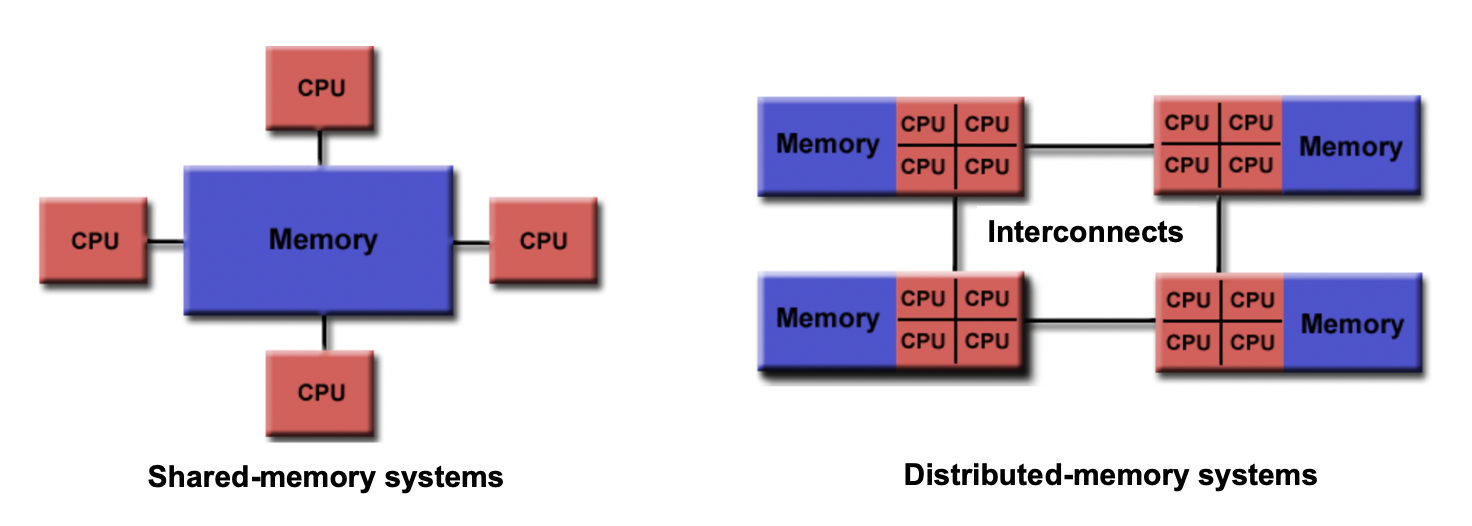
Depending upon what kind of memory a computer has, the parallelization approach of a code could vary. For example, in a distributed memory platform, when a CPU core needs data from its private memory, it is fast to get it. But, if it requires access to a data that resides in the private memory of another CPU core then it requires a ‘communication’ protocol and data access becomes slower.
Similar situation arises for GPU coding too. In this case, the CPU is generally called the host and the GPUs are called the devices. When we submit a GPU job, it is launched in the CPU (host) which in turn directs it to be executed by the GPUs (devices). While doing these calculations, data is copied from CPU memory to the GPU’s and then processed. After the GPU finishes a calculation, the result is copied back from the GPU to CPU. This communication is expensive and it could significantly slow down a calculation if care is not taken to minimize it. We’ll see later in this tutorial that communication is a major bottleneck in many calculations and we need to devise strategies to reduce the related overhead.
In shared memory platforms, the memory is being shared by all the processors. In this case, the processors communicate with each other directly through the shared memory…but we need to take care that the access the memory in the right order!
Parallelizing an application
When we say that we parallelize an application, we actually mean we devise a strategy that divides the whole job into pieces and assign each piece to a worker (CPU core or GPU) to help solve. This parallelization strategy depends heavily on the memory structure. For example, if we want to use OpenMP, it provides a thread level parallelism that is well-suited for a shared memory platform, but you can not use it in a distributed memory system. For a distributed memory system, you need a way to communicate between workers (a message passing protocol), like MPI.
Multithreading
If we think of a process as an instance of your application, multithreading is a shared memory parallelization approach which allows a single process to contain multiple threads which share the process’s resources but work relatively independently. OpenMP and CUDA are two very popular multithreading execution models that you may have heard of. OpenMP is generally used for multi-core/many-core CPUs and CUDA is used to utilize threading for GPUs.
The two main parallelization strategies are data parallelism and task parallelism. In data parallelism, some set of tasks are performed by each core using different subsets of the same data. Task parallelism is when we can decompose the larger task into multiple independent sub-tasks, each of which we then assign to different cores. A simple graphical representation is given below:
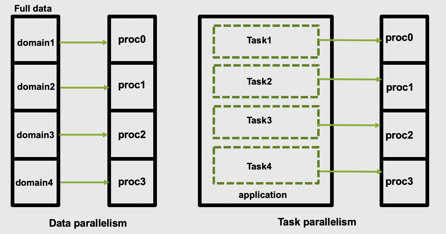
As application users, we need to know if our application actually offers control over which parallelization methods (and tools) we can use. If so, we then need to figure out how to make the right choices based on our use case and the hardware we have available to us.
Popular parallelization strategies
Data parallelism is conceptually easy to map to distributed memory, and it is the most commonly found choice on HPC systems. The main parallelization technique one finds is the domain decomposition method. In this approach, the global domain is divided into many sub-domains and then each sub-domain is assigned to a processor.
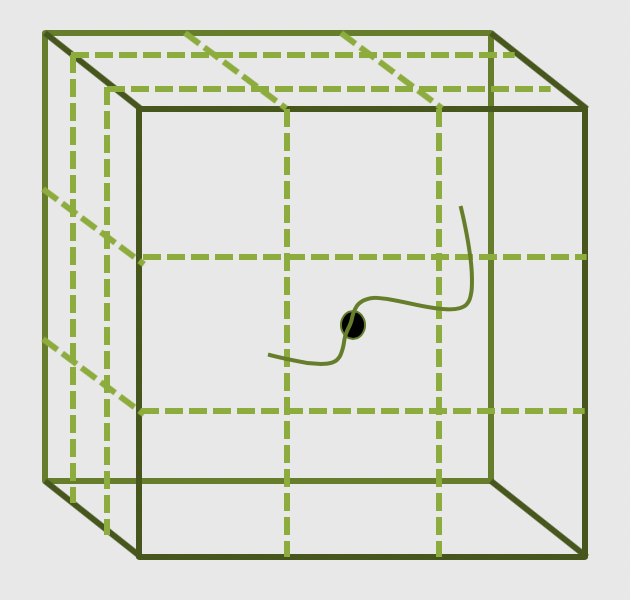
If your computer has N physical
processors, you could initiate
N MPI processes on your computer. This means each sub-domain is handled by an MPI process
and usually the domains communicate with their “closest” neighbours to exchange information.
What is MPI?
A long time before we had smart phones, tablets or laptops, compute clusters were already around and consisted of interconnected computers that had about enough memory to show the first two frames of a movie (2 x 1920 x 1080 x 4 Bytes = 16 MB). However, scientific problems back than were demanding more and more memory (as they are today). To overcome the lack of adequate memory, specialists from academia and industry came up with the idea to consider the memory of several interconnected compute nodes as one. They created a standardized software that synchronizes the various states of memory through the network interfaces between the client nodes during the execution of an application. With this performing large calculations that required more memory than each individual node can offer was possible.
Moreover, this technique of passing messages (hence Message Passing Interface or MPI) on memory updates in a controlled fashion allow us to write parallel programs that are capable of running on a diverse set of cluster architectures.(Reference: https://psteinb.github.io/hpc-in-a-day/bo-01-bonus-mpi-for-pi/ )
In addition to MPI, some applications also support thread level parallelism (through, for example OpenMP directives) which can offer additional parallelisation within a subdomain. The basic working principle in OpenMP is based the “Fork-Join” model, as shown below.
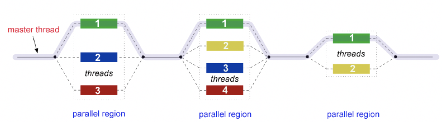
In the ‘Fork-Join’ model, there exists a master thread which “fork”s into multiple threads. Each of these forked-threads executes a part of the whole job and when all the threads are done with their assigned jobs, these threads join together again. Typically, the number of threads is equal to the number of available cores, but this can be influenced by the application or the user at run-time.
Using the maximum possible threads on a node may not always provide the best performance. It depends on many factors and, in some cases,the MPI parallelization strategy is so strongly integrated that it almost always offers better performance than the OpenMP based thread-level parallelism.
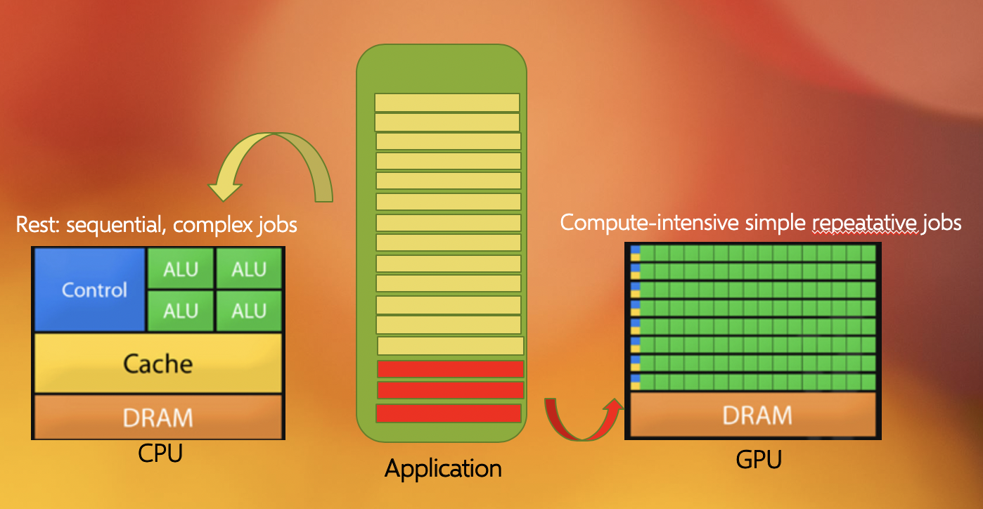
Another commonly found parallelization strategy is to use GPUs (with the more general term being an accelerator). GPUs work together with the CPUs. A CPU is specialized to perform complex tasks (like making decisions), while a GPU is very efficient in doing simple, repetitive, low level tasks. This functional difference between a GPU and CPU could be attributed to the massively parallel architecture that a GPU possesses. A modern CPU has relatively few cores which are well optimized for performing sequential serial jobs. On the contrary, a GPU has thousands of cores that are highly efficient at doing simple repetitive jobs in parallel. See below on how a CPU and GPU works together.
Using all available resources
Say you’ve actually got a powerful desktop with multiple CPU cores and a GPU at your disposal, what are good options for leveraging them?
- Utilising MPI (Message Passing Interface)
- Utilising OpenMP (Open Multi-Processing)
- Using performance enhancing libraries or plugins
- Use GPUs instead of CPUs
- Splitting code up into smaller individual parts
Solution
- Yes, MPI can enable you to split your code into multiple processes distributed over multiple cores (and even multiple computers), known as parallel programming. This won’t help you to use the GPU though.
- Yes, like MPI this is also parallel programming, but deals with threads instead of processes, by splitting a process into multiple threads, each thread using a single CPU core. OpenMP can potentially also leverage the GPU.
- Yes, that is their purpose. However, different libraries/plugins run on different architectures and with different capabilities, in this case you need something that will leverage the additional cores and/or the GPU for you.
- Yes, GPUs are better at handling multiple simple tasks, whereas a CPU is better at running complex singular tasks quickly.
- It depends, if you have a simulation that needs to be run from start to completion, then splitting the code into segments won’t be of any benefit and will likely waste compute resources due to the associated overhead. If some of the segments can be run simultaneously or on different hardware then you will see benefit…but it is usually very hard to balance this.
Key Points
OpenMP works on a single node, MPI can work on multiple nodes
Benchmarking and Scaling
Overview
Teaching: 15 min
Exercises: 15 minQuestions
What is benchmarking?
How do I do a benchmark?
What is scaling?
How do I perform a scaling analysis?
Objectives
Be able to perform a benchmark analysis of an application
Be able to perform a scaling analysis of an application
What is benchmarking?
To get an idea of what we mean by benchmarking, let’s take the example of a sprint athlete. The athlete runs a predetermined distance on a particular surface, and a time is recorded. Based on different conditions, such as how dry or wet the surface is, or what the surface is made of (grass, sand, or track) the times of the sprinter to cover a distance (100m, 200m, 400m etc) will differ. If you know where the sprinter is running, and what the conditions were like, when the sprinter sets a certain time you can cross-correlate it with the known times associated with certain surfaces (our benchmarks) to judge how well they are performing.
Benchmarking in computing works in a similar way: it is a way of assessing the performance of a program (or set of programs), and benchmark tests are designed to mimic a particular type of workload on a component or system. They can also be used to measure differing performance across different systems. Usually codes are tested on different computer architectures to see how a code performs on each one. Like our sprinter, the times of benchmarks depends on a number of things: software, hardware or the computer itself and it’s architecture.
Case study: Benchmarking with LAMMPS
As an example, let’s create some benchmarks for you to compare the performance of some ‘standard’ systems in LAMMPS. Using a ‘standard’ system is a good idea as a first attempt, since we can measure our benchmarks against (published) information from others. Knowing that our installation is “sane” is a critical first step before we embark on generating our own benchmarks for our own use case.
Installing your own software vs. system-wide installations
Whenever you get access to an HPC system, there are usually two ways to get access to software: either you use a system-wide installation or you install it yourself. For widely used applications, it is likely that you should be able to find a system-wide installation. In many cases using the system-wide installation is the better option since the system administrators will (hopefully) have configured the application to run optimally for that system. If you can’t easily find your application, contact user support for the system to help you.
You should still check the benchmark case though! Sometimes administrators are short on time or background knowledge of applications and do not do thorough testing.
As an example, we will start with the simplest Lennard-Jones (LJ) system as provided in
the bench directory of the LAMMPS distribution. You will also be given another
example with which you can follow the same workflow and compare your results with some
‘known’ benchmark.
Running a LAMMPS job on an HPC system
Can you list the bare minimum files that you need to schedule a LAMMPS job on an HPC system?
Solution
For running a LAMMPS job, we need:
- an input file
- a job submission file - in general, each HPC system uses a resource manager (frequently called queueing system) to manage all the jobs. Two popular ones are PBS and SLURM.
Optional files include:
- Empirical potential file
- Data file
These optional files are only required when the empirical potential model parameters and the molecular coordinates are not defined within the LAMMPS input file.
The input file we need for the LJ-system is reproduced below:
# 3d Lennard-Jones melt

variable	x index 1
variable	y index 1
variable	z index 1

variable	xx equal 20*$x
variable	yy equal 20*$y
variable	zz equal 20*$z

units		lj
atom_style	atomic

lattice		fcc 0.8442
region		box block 0 ${xx} 0 ${yy} 0 ${zz}
create_box	1 box
create_atoms	1 box
mass		1 1.0

velocity	all create 1.44 87287 loop geom

pair_style	lj/cut 2.5
pair_coeff	1 1 1.0 1.0 2.5

neighbor	0.3 bin
neigh_modify	delay 0 every 20 check no

fix		1 all nve

run		100
The timing information for this run with both 1 and 4 processors is also provided with the LAMMPS distribution. To do an initial benchmark our installation it would be wise to run the test case with the same number of processors in order to compare with the timing information provided by LAMMPS.
Let us now create a job file (sometimes called a batch file) to submit a job for a larger test case. Writing a job file from scratch is error prone. Many computing sites offer a number of example job scripts to let you get started. We’ll do the same and provide you with an example , but created specifically for our LAMMPS use case.
First we need to tell the batch system what resources we need:
#!/bin/bash -x

# Ask for 2 nodes of resources for an MPI job for 10 minutes

#SBATCH --account=ecam
#SBATCH --nodes=2
#SBATCH --ntasks-per-node=24
#SBATCH --output=mpi-out.%j
#SBATCH --error=mpi-err.%j
#SBATCH --time=00:10:00

# Let's use the devel partition for faster queueing time since we have a tiny job.
# (For a more substantial job we should use --partition=batch)

#SBATCH --partition=devel
in this case, we’ve asked for all the cores on 2 nodes of the system for 5 minutes.
Next we should tell it about the environment we need to run in. In most modern HPC systems,
package specific environment variables are loaded or unloaded using environment
modules. A module is a self-contained description of
a software package - it contains the settings required to run a software package and,
usually, encodes required dependencies on other software packages. See below for an
example set of module commands to load LAMMPS for this course:
# Prepare the execution environment
module purge
module use /usr/local/software/jureca/OtherStages
module load Stages/Devel-2019a
module load intel-para/2019a
module load LAMMPS/3Mar2020-Python-3.6.8-kokkos
And finally we tell it how to actually run the LAMMPS executable on the system. If we were using a single CPU core, we can invoke LAMMPS directly with
lmp -in in.lj
but in our case we are interested in using the MPI runtime across 2 nodes. On our system
we will use the ParaStation MPI implementation using
srun to launch the MPI processes. Let’s see how that looks
like for our current use case (with in.lj as the input file):
# Run our application ('srun' handles process distribution)
srun lmp -in in.lj
Now let’s put all that together to make our job script:
#!/bin/bash -x

# Ask for 2 nodes of resources for an MPI job for 10 minutes

#SBATCH --account=ecam
#SBATCH --nodes=2
#SBATCH --ntasks-per-node=24
#SBATCH --output=mpi-out.%j
#SBATCH --error=mpi-err.%j
#SBATCH --time=00:10:00

# Let's use the devel partition for faster queueing time since we have a tiny job.
# (For a more substantial job we should use --partition=batch)

#SBATCH --partition=devel

# Prepare the execution environment
module purge
module use /usr/local/software/jureca/OtherStages
module load Stages/Devel-2019a
module load intel-para/2019a
module load LAMMPS/3Mar2020-Python-3.6.8-kokkos

# Run our application ('srun' handles process distribution)
srun lmp -in in.lj
Edit a submission script for a LAMMPS job
Duplicate the job script we just created so that we have versions that will run on 1 core and 4 cores.
Make a new directories (called
4core_ljand1core_lj) and for each directory copy inside your input file and the relevant job script. For each case, enter that directory (so that all output from your job is stored in the same place) and run the job script on JURECA.Solution
Our single core version is
#!/bin/bash -x

# Ask for 1 nodes (1 CPU) of resources for an MPI job for 10 minutes

#SBATCH --account=ecam
#SBATCH --nodes=1
#SBATCH --ntasks-per-node=1
#SBATCH --output=mpi-out.%j
#SBATCH --error=mpi-err.%j
#SBATCH --time=00:10:00

# Let's use the devel partition for faster queueing time since we have a tiny job.
# (For a more substantial job we should use --partition=batch)

#SBATCH --partition=devel

# Prepare the execution environment
module purge
module use /usr/local/software/jureca/OtherStages
module load Stages/Devel-2019a
module load intel-para/2019a
module load LAMMPS/3Mar2020-Python-3.6.8-kokkos

# Run our application ('srun' handles process distribution)
srun lmp -in in.lj
and our 4 core version is
#!/bin/bash -x

# Ask for 1 nodes (4 CPUs) of resources for an MPI job for 10 minutes

#SBATCH --account=ecam
#SBATCH --nodes=1
#SBATCH --ntasks-per-node=4
#SBATCH --output=mpi-out.%j
#SBATCH --error=mpi-err.%j
#SBATCH --time=00:10:00

# Let's use the devel partition for faster queueing time since we have a tiny job.
# (For a more substantial job we should use --partition=batch)

#SBATCH --partition=devel

# Prepare the execution environment
module purge
module use /usr/local/software/jureca/OtherStages
module load Stages/Devel-2019a
module load intel-para/2019a
module load LAMMPS/3Mar2020-Python-3.6.8-kokkos

# Run our application ('srun' handles process distribution)
srun lmp -in in.lj
Understanding the output files
Let us now look at the output files. Here, three files have been created: log.lammps,
mpi-out.xxxxx, and mpi-err.xxxxx. Among these three, mpi-out.xxxxx is mainly to
capture the screen output that would have been generated during the job execution. The purpose
of the mpi-err.xxxxx file is to log entries if there is any error (and sometimes other
information) that occurred during
run-time. The one that is created by LAMMPS is called log.lammps. Note that LAMMPS
overwrites the default log.lammps file with every execution, but the information we
are concerned with there is also stored in our mpi-out.xxxxx file.
Once you open log.lammps, you will notice that it contains most of the important
information starting from the LAMMPS version (in our case we are using
3Mar2020), the number of processors used for runs,
the processor lay out, thermodynamic steps, and some timings. The header of your
log.lammps file
should be somewhat similar to this:
LAMMPS (18 Feb 2020)
OMP_NUM_THREADS environment is not set. Defaulting to 1 thread. (src/comm.cpp:94)
using 1 OpenMP thread(s) per MPI task
Note that it tells you about the LAMMPS version, and OMP_NUM_THREADS which is one of
the important environment variables we need to know about to leverage OpenMP. For
now, we’ll focus mainly on the timing
information provided in this file.
When the run concludes, LAMMPS prints the final thermodynamic state and a total run time for the simulation. It also appends statistics about the CPU time and storage requirements for the simulation. An example set of statistics is shown here:
Loop time of 1.76553 on 1 procs for 100 steps with 32000 atoms

Performance: 24468.549 tau/day, 56.640 timesteps/s
100.0% CPU use with 1 MPI tasks x 1 OpenMP threads

MPI task timing breakdown:
Section |  min time  |  avg time  |  max time  |%varavg| %total
---------------------------------------------------------------
Pair    | 1.5244     | 1.5244     | 1.5244     |   0.0 | 86.34
Neigh   | 0.19543    | 0.19543    | 0.19543    |   0.0 | 11.07
Comm    | 0.016556   | 0.016556   | 0.016556   |   0.0 |  0.94
Output  | 7.2241e-05 | 7.2241e-05 | 7.2241e-05 |   0.0 |  0.00
Modify  | 0.023852   | 0.023852   | 0.023852   |   0.0 |  1.35
Other   |            | 0.005199   |            |       |  0.29

Nlocal:    32000 ave 32000 max 32000 min
Histogram: 1 0 0 0 0 0 0 0 0 0
Nghost:    19657 ave 19657 max 19657 min
Histogram: 1 0 0 0 0 0 0 0 0 0
Neighs:    1.20283e+06 ave 1.20283e+06 max 1.20283e+06 min
Histogram: 1 0 0 0 0 0 0 0 0 0

Total # of neighbors = 1202833
Ave neighs/atom = 37.5885
Neighbor list builds = 5
Dangerous builds not checked
Total wall time: 0:00:01
Useful keywords to search for include:
-
Loop time:This shows the total wall-clock time for the simulation to run. (source: LAMMPS manual)The following command can be used to extract this the relevant line from
log.lammps:grep "Loop time" log.lammps -
Performance: This is provided for convenience to help predict how long it will take to run a desired physical simulation. (source: LAMMPS manual)
Use the following command line to extract line (we will use the value in units of
tau/day):grep "Performance" log.lammps -
CPU use: This provides the CPU utilization per MPI task; it should be close to 100% times the number of OpenMP threads (or 1 of not using OpenMP). Lower numbers correspond to delays due to file I/O or insufficient thread utilization. (source: LAMMPS manual)
Use the following command line to extract the relevant line:
grep "CPU use" log.lammps -
Timing Breakdown Next, we’ll discuss about the timing breakdown table for CPU runtime. If we try the following command;
# extract 8 lines after the occurrence of the "breakdown"
grep -A 8 "breakdown" log.lammps
you should see output similar to the following:
MPI task timing breakdown:
Section |  min time  |  avg time  |  max time  |%varavg| %total
---------------------------------------------------------------
Pair    | 1.5244     | 1.5244     | 1.5244     |   0.0 | 86.34
Neigh   | 0.19543    | 0.19543    | 0.19543    |   0.0 | 11.07
Comm    | 0.016556   | 0.016556   | 0.016556   |   0.0 |  0.94
Output  | 7.2241e-05 | 7.2241e-05 | 7.2241e-05 |   0.0 |  0.00
Modify  | 0.023852   | 0.023852   | 0.023852   |   0.0 |  1.35
Other   |            | 0.005199   |            |       |  0.29
The above table shows the times taken by the major categories of a LAMMPS run. A brief description of these categories has been provided in the run output section of the LAMMPS manual:
- Pair = non-bonded force computations
- Bond = bonded interactions: bonds, angles, dihedrals, impropers
- Kspace = long-range interactions: Ewald, PPPM, MSM
- Neigh = neighbor list construction
- Comm = inter-processor communication of atoms and their properties
- Output = output of thermodynamic info and dump files
- Modify = fixes and computes invoked by fixes
- Other = all the remaining time
This is very useful in the sense that it helps you to identify where you spend most of your computing time (and so help you know what you should be targeting)! It will discussed later in more detail.
Now run a benchmark…
From the jobs that you ran previously, extract the loop times for your runs and see how they compare with the LAMMPS standard benchmark and with the performance for two other HPC systems.
HPC system 1 core (sec) 4 core (sec) LAMMPS 2.26185 0.635957 HPC 1 2.24207 0.592148 HPC 2 1.76553 0.531145 MY HPC ? ? Why might these results differ?
Scaling
Scaling behaviour in computation is centred around the effective use of resources as you scale up the amount of computing resources you use. An example of “perfect” scaling would be that when we use twice as many CPUs, we get an answer in half the time. “Bad” scaling would be when the answer takes only 10% less time when we double the CPUs. This example is one of strong scaling, where the workload doesn’t change as we increase our resources.
Plotting strong scalability
Use the original job script for 2 nodes and run it on JURECA.
Now that you have results for 1 core, 4 cores and 2 nodes, create a scalability plot with the number of CPU cores on the X-axis and the loop times on the Y-axis (use your favourite plotting tool, an online plotter or even pen and paper).
Are you close to “perfect” scalability?
Weak scaling
For weak scaling, we want usually want to increase our workload without increasing our walltime, and we do that by using additional resources. To consider this in more detail, let’s head back to our chefs again from the previous episode, where we had more people to serve but the same amount of time to do it in.
We hired extra chefs who have specialisations but let us assume that they are all bound by secrecy, and are not allowed to reveal to you what their craft is, pastry, meat, fish, soup, etc. You have to find out what their specialities are, what do you do? Do a test run and assign a chef to each course. Having a worker set to each task is all well and good, but there are certain combinations which work and some which do not, you might get away with your starter chef preparing a fish course, or your lamb chef switching to cook beef and vice versa, but you wouldn’t put your pastry chef in charge of the main meat dish, you leave that to someone more qualified and better suited to the job.
Scaling in computing works in a similar way, thankfully not to that level of detail where one specific core is suited to one specific task, but finding the best combination is important and can hugely impact your code’s performance. As ever with enhancing performance, you may have the resources, but the effective use of the resources is where the challenge lies. Having each chef cooking their specialised dishes would be good weak scaling: an effective use of your additional resources. Poor weak scaling will likely result from having your pastry chef doing the main dish.
Key Points
Benchmarking is a way of assessing the performance of a program or set of programs
The
log.lammpsfile shows important information about the timing, processor layout, etc. which you can use to record your benchmarkScaling concerns the effective use of computational resources. Two types are typically discussed: strong scaling (where we increase the compute resources but keep the problem size the same) and weak scaling (where we increase the problem size in proportion to our increase of compute resources
Bottlenecks in LAMMPS
Overview
Teaching: 40 min
Exercises: 45 minQuestions
How can I identify the main bottlenecks in LAMMPS?
How do I come up with a strategy for finding the best optimisation?
What is load balancing?
Objectives
Learn how to analyse timing data in LAMMPS and determine bottlenecks
Earlier, you have learnt the basic philosophies behind various parallel computing methods (like MPI, OpenMP and CUDA). LAMMPS is a massively-parallel molecular dynamics package that is primarily designed with MPI-based domain decomposition as its main parallelization strategy. It supports all of the other parallelization techniques through the use of appropriate accelerator packages on the top of the intrinsic MPI-based parallelization.
So, is the only thing that needs to be done is decide on which accelerator package to use? Before using any accelerator package to speedup your runs, it is always wise to identify performance bottlenecks. The term “bottleneck” refers to specific parts of an application that are unable to keep pace with the rest of the calculation, thus slowing overall performance.
Therefore, you need to ask yourself these questions:
- Are my runs slower than expected?
- What is it that is hindering us getting the expected scaling behaviour?
Identify bottlenecks
Identifying (and addressing) performance bottlenecks is important as this could save you a lot of computation time and resources. The best way to do this is to start with a reasonably representative system having a modest system size and run for a few hundred/thousand timesteps.
LAMMPS provides a timing breakdown table printed at the end of log file and also within the screen output file generated at the end of each LAMMPS run. The timing breakdown table has already been introduced in the previous episode but let’s take a look at it again:
MPI task timing breakdown:
Section |  min time  |  avg time  |  max time  |%varavg| %total
---------------------------------------------------------------
Pair    | 1.5244     | 1.5244     | 1.5244     |   0.0 | 86.34
Neigh   | 0.19543    | 0.19543    | 0.19543    |   0.0 | 11.07
Comm    | 0.016556   | 0.016556   | 0.016556   |   0.0 |  0.94
Output  | 7.2241e-05 | 7.2241e-05 | 7.2241e-05 |   0.0 |  0.00
Modify  | 0.023852   | 0.023852   | 0.023852   |   0.0 |  1.35
Other   |            | 0.005199   |            |       |  0.29
Note that %total of the timing is giving for a range of different parts of the
calculation. In the following section, we will work on a few examples and try to
understand how to identify bottlenecks from this output. Ultimately, we will try to find
a way to minimise the walltime by adjusting the balance between
Pair, Neigh, Comm and the other parts of the calculation.
To get a feeling for this process, let us start with a Lennard-Jones (LJ) system. We’ll study two systems: the first one is with 4,000 atoms only; and the other one would be quite large, almost 10 million atoms. The following input file is for a LJ-system with an fcc lattice:
# 3d Lennard-Jones melt
variable        x index 10
variable        y index 10
variable        z index 10
variable        t index 1000

variable        xx equal 1*$x
variable        yy equal 1*$y
variable        zz equal 1*$z

variable        interval equal $t/2

units           lj
atom_style      atomic

lattice         fcc 0.8442
region          box block 0 ${xx} 0 ${yy} 0 ${zz}
create_box      1 box
create_atoms    1 box
mass            1 1.0

velocity        all create 1.44 87287 loop geom

pair_style      lj/cut 2.5
pair_coeff      1 1 1.0 1.0 2.5

neighbor        0.3 bin
neigh_modify    delay 0 every 20 check no

fix             1 all nve

thermo ${interval}
thermo_style custom step time  temp press pe ke etotal density
run             $t
We can vary the system size (i.e. number of atoms) by assigning appropriate
values to the variables x, y, and z at the beginning of the input file.
The length of the run can be decided by the
variable t. We’ll choose two different system sizes here: the one given is tiny just
having 4000 atoms (x = y = z = 10, t = 1000). If we take this input and modify it
such that x = y = z = 140 the other one would be huge
containing about 10 million atoms.
Important!
For many of these exercises, the exact modifications to job scripts that you will need to implement are system specific. Check with your instructor or your HPC institution’s helpdesk for information specific to your HPC system.
Also remember that after each execution the
log.lammpsfile in the current directory may be overwritten but you will still have the information we require in thempi-out.XXXXXfile corresponding to the executed job.
Example timing breakdown for 4000 atoms LJ-system
Using your previous job script for a a serial run (i.e. on a single core), replace the input file with the one for the small system (having 4000 atoms) and run it on the HPC system.
Take a look at the resulting timing breakdown table and discuss with your neighbour what you think you should target to get a performance gain.
Solution
Let us have a look at an example of the timing breakdown table.
MPI task timing breakdown:
Section |  min time  |  avg time  |  max time  |%varavg| %total
---------------------------------------------------------------
Pair    | 12.224     | 12.224     | 12.224     |   0.0 | 84.23
Neigh   | 1.8541     | 1.8541     | 1.8541     |   0.0 | 12.78
Comm    | 0.18617    | 0.18617    | 0.18617    |   0.0 |  1.28
Output  | 7.4148e-05 | 7.4148e-05 | 7.4148e-05 |   0.0 |  0.00
Modify  | 0.20477    | 0.20477    | 0.20477    |   0.0 |  1.41
Other   |            | 0.04296    |            |       |  0.30
The last
%totalcolumn in the table tells about the percentage of the total loop time is spent in this category. Note that most of the CPU time is spent onPairpart (~84%), about ~13% on theNeighpart and the rest of the things have taken only 3% of the total simulation time. So, in order to get a performance gain, the common choice would be to find a way to reduce the time taken by thePairpart since improvements there will have the greatest impact on the overall time. Often OpenMP or using a GPU can help us to achieve this…but not always! It very much depends on the system that you are studying (the pair styles you use in your calculation need to be supported).Serial timing breakdown for 10 million atoms LJ-system
The following table shows an example timing breakdown for a serial run of the large, 10 million atom system. Note that, though the absolute time to complete the simulation has increased significantly (it now takes about 1.5 hours), the distribution of
%totalremains roughly the same.MPI task timing breakdown: Section | min time | avg time | max time |%varavg| %total --------------------------------------------------------------- Pair | 7070.1 | 7070.1 | 7070.1 | 0.0 | 85.68 Neigh | 930.54 | 930.54 | 930.54 | 0.0 | 11.28 Comm | 37.656 | 37.656 | 37.656 | 0.0 | 0.46 Output | 0.1237 | 0.1237 | 0.1237 | 0.0 | 0.00 Modify | 168.98 | 168.98 | 168.98 | 0.0 | 2.05 Other | | 43.95 | | | 0.53
Effects due to system size on resource used
Different sized systems might behave differently as we increase our resource usage since they will have different distributions of work among our available resources.
Analysing the small system
Below is an example timing breakdown for 4000 atoms LJ-system with 40 MPI ranks
MPI task timing breakdown:
Section |  min time  |  avg time  |  max time  |%varavg| %total
---------------------------------------------------------------
Pair    | 0.24445    | 0.25868    | 0.27154    |   1.2 | 52.44
Neigh   | 0.045376   | 0.046512   | 0.048671   |   0.3 |  9.43
Comm    | 0.16342    | 0.17854    | 0.19398    |   1.6 | 36.20
Output  | 0.0001415  | 0.00015538 | 0.00032134 |   0.0 |  0.03
Modify  | 0.0053594  | 0.0055818  | 0.0058588  |   0.1 |  1.13
Other   |            | 0.003803   |            |       |  0.77
Can you discuss any observations that you can make from the above table? What could be the rationale behind such a change of the
%totaldistribution among various categories?Solution
The first thing that we notice in this table is that when we use 40 MPI processes instead of 1 process, percentage contribution of the
Pairpart to the total looptime has come down to about ~52% from 84%, similarly for theNeighpart also the percentage contribution reduced considerably. The striking feature is that theCommis now taking considerable part of the total looptime. It has increased from ~1% to nearly 36%. But why?We have 4000 total atoms. When we run this with 1 core, this handles calculations (i.e. calculating pair terms, building neighbour list etc.) for all 4000 atoms. Now when you run this with 40 MPI processes, the particles will be distributed among these 40 cores “ideally” equally (if there is no load imbalance (see below)). These cores then do the calculations in parallel, sharing information when necessary. This leads to the speedup. But this comes at a cost of communication between these MPI processes. So, communication becomes a bottleneck for such systems where you have a small number of atoms to handle and many workers to do the job. This implies that you really don’t need to waste your resource for such a small system.
Analysing the large system
Now consider the following breakdown table for the 10 million atom system with 40 MPI-processes. You can see that in this case, the
Pairterm is still dominating the table. Discuss about the rationale behind this.MPI task timing breakdown: Section | min time | avg time | max time |%varavg| %total --------------------------------------------------------------- Pair | 989.3 | 1039.3 | 1056.7 | 55.6 | 79.56 Neigh | 124.72 | 127.75 | 131.11 | 10.4 | 9.78 Comm | 47.511 | 67.997 | 126.7 | 243.1 | 5.21 Output | 0.0059468 | 0.015483 | 0.02799 | 6.9 | 0.00 Modify | 52.619 | 59.173 | 61.577 | 25.0 | 4.53 Other | | 12.03 | | | 0.92Solution
In this case, the system size is enormous. Each core will have enough atoms to deal with so it remains busy in computing and the time taken for the communication is still much smaller as compared to the “real” calculation time. In such cases, using many cores is actually beneficial.
One more thing to note here is the second last column
%varavg. This is the percentage by which the max or min varies from the average value. A value near to zero implies perfect load balance, while a large value indicated load imbalance. So, in this case, there is a considerable amount of load imbalance specially for theCommandPairpart. To improve the performance, one may like to explore a way to minimize load imbalance (but unfortunately we won’t have time to cover this topic).
Scalability
Since we have information about the timings for different components of the calculation, we can perform a scalability study for each of the components.
Investigating scalability on a number of nodes
Make a copy of the example input modified to run the large system (
x = y = z = 140).Now run the two systems using all the cores available in a single node and then run with more nodes (2, 4) with full capacity and note how this timing breakdown varies rapidly. While running with multiple cores, we’re using only MPI only as parallelization method.
You can use the job scripts from the previous episode as a starting point.
Using the
log.lammps(ormpi-out.XXXXX) files, write down the speedup factor for thePair,Commandwalltimefields in the timing breakdowns. Use the below formula to calculate speedup.(Speedup factor) = 1.0 / ( (Time taken by N nodes) / (Time taken by 1 node) )Note here how we have uses a node for our baseline unit of measurement (rather than a single processor) since running the serial case would take too long.
Using a simple pen and paper, make a plot of the speedup factor on the y-axis and number of processors on the x-axis for each of these fields.
What are your observations about this plot? Which fields show a good speedup factor? Discuss what could be a good approach in fixing this.
Solution
You should have noticed that
Pairshows almost perfect linear scaling, whereasCommshows poor scalability. and the total walltime also suffers from the poor scalability when running with more number of cores.However, remember this is a pretty small sample size, to do a definitive study more nodes/cores would need to be utilised.
MPI vs OpenMP
By now you should have developed some understanding on how can you use the timing breakdown table to identify performance bottlenecks in a LAMMPS run. But identifying the bottleneck is not enough, you need to decide what strategy would ‘probably’ be more sensible to apply in order to unblock the bottlenecks. The usual method of speeding up a calculation is to employ some form of parallelization. We have already discussed in a previous episode that there are many ways to implement parallelism in a code.
MPI based parallelism using domain decomposition lies at the core of LAMMPS. Atoms in each domain are associated to 1 MPI task. This domain decomposition approach comes with a cost however, keeping track and coordinating things among these domains requires communication overhead. It could lead to significant drop in performance if you have limited communication bandwidth, a slow network, or if you wish to scale to a very large number of cores.
While MPI offers domain based parallelization, one can also use parallelization over particles. This can, for example, be done using OpenMP which is a different parallelization paradigm based on threading. Moreover, OpenMP parallelization is orthogonal to MPI parallelization which means you can use them together. OpenMP also comes with an overhead: starting and stopping OpenMP takes compute time; OpenMP also needs to be careful about how it handles memory, the particular use case also impacts the efficiency. Remember that, in general, a threaded parallelization method in LAMMPS may not be as efficient as MPI unless you have situations where domain decomposition is no longer efficient (we will see below how to recognise such situations).
Let us discuss a few situations:
- The LJ-system with 4000 atoms (discussed above): Communication bandwidth with more
MPI processes. When you have too few atoms per domain, at some point LAMMPS will
not scale, and may even run slower, if you use more processors via
MPI only. With a pair style like
lj/cutthis will happen at a rather small number of atoms. - The LJ-system with with 10M atoms (discussed above): More atoms per processor, still communication is not a big deal in this case. This happens because you have a dense, homogeneous, well behaved system with a sufficient number of atoms, so that the MPI parallelization can be at its most efficient.
- Inhomogeneous or slab systems: In systems where there could be lots of empty spaces
in the simulation cell, the number of atoms handled across these domains will vary
a lot resulting in severe load balancing issue. While some of the domains will be
over-subscribed, some of them will remain under-subscribed causing these domains
(cores) to be less efficient in terms of performance. Often this could be improved by
using the
processorkeyword in a smart fashion, beyond that, there are the load balancing commands (balancecommand) and changing the communication using recursive bisecting and decomposition strategy. This might not help always since some of the systems are pathological. In such cases, a combination of MPI and OpenMP could often provide better parallel efficiency as this will result in larger subdomains for the same number of total processors and if you parallelize over particles using OpenMP threads, generally it does not hamper load balancing in a significant way. So, a sensible mix of MPI, OpenMP and thebalancecommand can help you to fetch better performance from the same hardware. - MD problems: For these, we need to deal with the calculation of electrostatic
interactions. Unlike the pair forces, electrostatic interactions are long range by
nature. To compute this long range interactions, very popular methods in MD are
ewaldandpppm. These long range solvers perform their computations in K-space. In case ofpppm, extra overhead results from the 3d-FFT, where as the Ewald method suffers from the poor \(O(N^\frac{3}{2})\) scaling, which will drag down the overall performance when you use more cores to do your calculation, even though Pair exhibits linear scaling. This is also a potential case where a hybrid run comprising of MPI and OpenMP might give you better performance and improve the scaling.
Let us now build some hands-on experience to develop some feeling on how this works.
Case study: Rhodopsin system
The following input file,
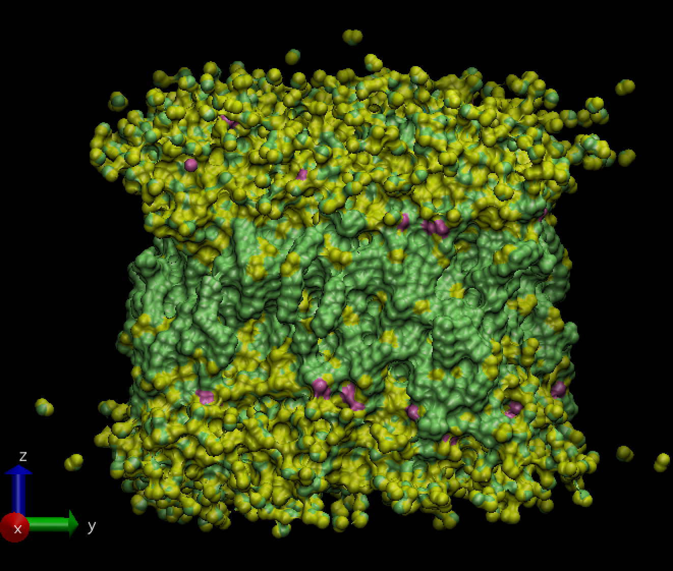
in.rhodo, is one of the inputs provided in the bench directory of the LAMMPS distribution (version7Aug2019):# Rhodopsin model variable x index 1 variable y index 1 variable z index 1 variable t index 2000 units real neigh_modify delay 5 every 1 atom_style full # atom_modify map hash bond_style harmonic angle_style charmm dihedral_style charmm improper_style harmonic pair_style lj/charmm/coul/long 8.0 10.0 pair_modify mix arithmetic kspace_style pppm 1e-4 read_data data.rhodo replicate $x $y $z fix 1 all shake 0.0001 5 0 m 1.0 a 232 fix 2 all npt temp 300.0 300.0 100.0 & z 0.0 0.0 1000.0 mtk no pchain 0 tchain 1 special_bonds charmm thermo 500 thermo_style multi timestep 2.0 run $tNote that this input file requires an additional data file
data.rhodo.Using this you can perform a simulation of an all-atom rhodopsin protein in solvated lipid bilayer with CHARMM force field, long-range Coulombics interaction via PPPM (particle-particle particle mesh) and SHAKE constraints. The box contains counter-ions and a reduced amount of water to make a 32000 atom system. The force cutoff for LJ force-field is 10.0 Angstroms, neighbor skin cutoff is 1.0 sigma, number of neighbors per atom is 440. NPT time integration is performed for 20,000 timesteps.
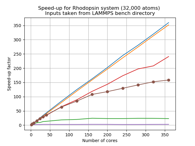
Let’s look at a scalability study of this system,
This was carried out on an Intel Skylake processor which has 2 sockets and 20 cores each, meaning 40 physical cores per node. Here jobs were run with 1, 4, 8, 16, 32, 40 processors, and then scaled up to 80, 120, 160, 200, 240, 280, 320, 360, 400 cores.
As we can see, similar to your own study,
PairandBondshow almost perfect linear scaling, whereasKspaceandCommshow poor scalability, and the total walltime also suffers from the poor scalability when running with more number of cores. This resembles situation 4 discussed above. A mix of MPI and OpenMP could be a sensible approach.
Load balancing
One important issue with MPI-based parallelization is that it can under-perform for systems with inhomogeneous distribution of particles, or systems having lots of empty space in them. It is pretty common that the evolution of simulated systems evolve over time to reflect such a case. This results in load imbalance. While some of the processors are assigned with finite number of particles to deal with for such systems, a few processors could have far less atoms (or none) to do any calculation and this results in an overall loss in parallel efficiency. This situation is more likely to expose itself as you scale up to a large large number of processors.
Let us take a look at another example from the LAMMPS bench directory with the input file
below which is run with
1 core (i.e., in serial) with x = y = z = 1, and t = 10,000.
variable        x index 1
variable        y index 1
variable        z index 1
variable        t index 10000

units           lj
atom_style      bond
atom_modify     map hash
special_bonds   fene

read_data       data.chain

replicate       $x $y $z

neighbor        0.4 bin
neigh_modify    every 1 delay 1

bond_style      fene
bond_coeff      1 30.0 1.5 1.0 1.0

pair_style      lj/cut 1.12
pair_modify     shift yes
pair_coeff      1 1 1.0 1.0 1.12

fix             1 all nve
fix             2 all langevin 1.0 1.0 10.0 904297

thermo          10000
timestep        0.012

run             $t
Example timing breakdown for system with low average number of neighbours
Section |  min time  |  avg time  |  max time  |%varavg| %total
---------------------------------------------------------------
Pair    | 20.665     | 20.665     | 20.665     |   0.0 | 18.24
Bond    | 6.9126     | 6.9126     | 6.9126     |   0.0 |  6.10
Neigh   | 57.247     | 57.247     | 57.247     |   0.0 | 50.54
Comm    | 4.3267     | 4.3267     | 4.3267     |   0.0 |  3.82
Output  | 0.000103   | 0.000103   | 0.000103   |   0.0 |  0.00
Modify  | 22.278     | 22.278     | 22.278     |   0.0 | 19.67
Other   |            | 1.838      |            |       |  1.62
Note that, in this case, the time spent in solving the
Pairpart is quite low as compared to theNeighpart. What do you think may have caused such an outcome?Solution
This kind of timing breakdown generally indicates either there is something wrong with the input or a very, very unusual system geometry. If you investigate the log file carefully, you would find that this is a system with a very short cutoff (1.12 sigma) resulting in on average less than 5 neighbors per atom (
Ave neighs/atom = 4.85891) and thus spending very little time on computing non-bonded forces.Being a sparse system, the necessity of rebuilding its neighbour lists is more frequent and this explains why the time spent of the
Neighpart is much more (about 50%) than thePairpart (~18%). On the contrary, the LJ-system is the extreme opposite. It is a relatively dense system having the average number of neighbours per atom nearly 37 (Ave neighs/atom = 37.4618). More computing operations are needed to decide the pair forces per atom (~84%), and less frequent would be the need to rebuild the neighbour list (~10%). So, here your system geometry is the bottleneck that causes the neighbour list building to happen too frequently and taking a significant part of the entire simulation time.
You can deal with load imbalance up to a certain extent using processors and balance
commands in LAMMPS. Detailed usage is given in the
LAMMPS manual. Unfortunately load balancing
is out of scope for this lesson since it is a somewhat complicated topic.
Key Points
The best way to identify bottlenecks is to run different benchmarks on a smaller system and compare it to a representative system
Effective load balancing is being able to distribute an equal amount of work across processes
Accelerating LAMMPS
Overview
Teaching: 30 min
Exercises: 90 minQuestions
What are the various options to accelerate LAMMPS?
What accelerator packages are compatible with which hardware?
How do I invoke a package in a LAMMPS run?
Objectives
Understand the different accelerator packages available in LAMMPS
Learn how to invoke the different accelerator packages across different hardwares
How can I accelerate LAMMPS performance?
There are two basic approaches to speed LAMMPS up. One is to use better algorithms for certain types of calculation, and the other is to use highly optimized codes via various “accelerator packages” for hardware specific platforms.
One popular example of the first approach is to use the Wolf summation method instead of the Ewald summation method for calculating long range Coulomb interactions effectively using a short-range potential. Similarly there are a few FFT schemes offered by LAMMPS and a user has to make a trade-off between accuracy and performance depending on their computational needs. This lesson is not aimed to discuss such types of algorithm-based speed-up of LAMMPS, instead we’ll focus on a few accelerator packages that are used to extract the most out of the available hardware of an HPC system.
There are five accelerator packages currently offered by LAMMPS. These are;
- OPT
- USER-INTEL
- USER-OMP
- GPU
- KOKKOS
Specialized codes contained in these packages help LAMMPS to perform well on the spectrum of architectures found in modern HPC platforms. Therefore, the next question that arises is: What hardware is supported by these packages?
Supported hardware
Here are some examples of the which packages support certain hardware:
Hardware Accelerator packages Multi-core CPUs OPT, USER-INTEL, USER-OMP, KOKKOS Intel Xeon Phi USER-INTEL, KOKKOS NVIDIA GPU GPU, KOKKOS
Within the limited scope of this tutorial, it is almost impossible to discuss all of the above packages in detail. The key point to understand is that, in all cases, the acceleration packages use multi-threading for parallelization, but how they do it and what architecture they can address differ.
The ONLY accelerator package that supports all kinds of hardware is KOKKOS. KOKKOS is a templated C++ library developed in Sandia National Laboratory and this helps to create an abstraction that allows a single implementation of a software application on different kinds of hardware. This will be discussed in detail in the next lesson.
In the meantime, we’ll touch a few key points about other accelerator packages to give you a feel about what these packages offer. To do this we will learn:
- how to invoke an accelerator package in a LAMMPS run
- how to gather data to compare the speedup with other LAMMPS runs.
Accelerator package overview
Precision
For many the accelerator packages you have the option to use
single,doubleormixedprecision. Precision means the amount of bytes that are used to store a number on a computer: the more bytes you use, the more precise the representation of a number you can have.doubleprecision uses double the amount of bytes assingleprecision. You should only use the precision that you need to, as higher precision comes with costs (more bytes for numbers means more work for the CPU, more storage and more bandwidth for communication).
mixedprecision is different in that it is implemented in an algorithm. It usually means you usesingleprecision when you can (to save CPU time and interconnect bandwidth) and double (or higher) precision when you have to (because you need numbers to a certain accuracy).
OPT package
- Only a handful of pair styles can be accelerated using this package (the list can be found here).
- Acceleration, in this case, is achieved by using a templated C++ library to reduce computational
overheads due to
iftests and other conditional code blocks.- This also provides better vectorization operations as compared to its regular CPU version.
- This generally offers 5-20% savings on computational cost on most machines
Effect on the timing breakdown table
We have discussed earlier that at the end of each run LAMMPS prints a timing breakdown table where it categorises the spent time into several categories (like
Pair,Bond,Kspace,Neigh,Comm,Output,Modify,Other). Can you make a justified guess about which of these category could be affected by the use of the OPT package?Solution
The
Paircomponent will see a reduction in cost since this accelerator package aims to work on the pair styles only.
USER-INTEL package
The USER-INTEL package supports single, double and mixed precision calculations.
Acceleration, in this case, is achieved in two different ways:
- Use vectorisation on multi-core CPUs
- Offload calculations of neighbour list and non-bonded interactions to Phi co-processors.
There are, however, a number of conditions:
- For using the offload feature, the (now outdated) Intel Xeon Phi coprocessors are required.
- For using vectorization feature, Intel compiler with version 14.0.1.106 or versions 15.0.2.044 and higher is required on both multi-core CPUs and Phi systems.
There are many LAMMPS features that are supported by this accelerator package, the list can be found here.
Performance enhancement using this package depends on many considerations, such as the
hardware that is available to you, the various styles that you are using in the input,
the size of your problem, and the selected precision. For example, if you are using a
pair style (say, reax) for which this is not implemented, its obvious that you are not
going to have a performance gain for the Pair part of the calculation. If the
majority of the computation time is coming from the Pair part then you are in trouble.
If you would like to know how much speedup you can expect to achieve using USER-INTEL, you can
take a look in the corresponding
LAMMPS documentation.
USER-OMP package
This accelerator package offers performance gain through optimisation and multi-threading via the OpenMP interface. In order to make the multi-threading functional, you will need multi-core CPUs and a compiler that supports multi-threading. If your compiler does not support multi-threading then also you can still use it as an optimized serial code.
A large sub-set of the LAMMPS routines can be used with this accelerator. A list of functionalities enabled with this package can be found here.
Generally, one can expect 5-20% performance boost when using this package even in serial! You should always test to figure out what the optimal number of OpenMP threads to use for a particular simulation is. Typically, the package gives better performance when used for lower numbers of threads, for example 2-4. It is important to remember that the MPI implementation in LAMMPS is so robust that you may almost always expect this to be more effective than using OpenMP on multi-core CPUs.
GPU package
Using the GPU package in LAMMPS, one can achieve performance gain by coupling GPUs to one or many CPUs. The package supports both CUDA (which is vendor specific) and OpenCL (which is an open standard) so it can be used on a variety of GPU hardware.
Calculations that require access to atomic data like coordinates, velocities, forces may suffer bottlenecks since at every step these data are communicated back and forth between the CPUs and GPUs. Calculations can be done in single, double or mixed precisions.
In case of the GPU package, computations are shared between CPUs and GPUs (unlike the KOKKOS package GPU implementation where the primary aim is to offload all of the calculations to the GPUs only). For example, asynchronous force calculations like pair vs bond/angle/dihedral/improper can be done simultaneously on GPUs and CPUs respectively. Similarly, for PPPM calculations the charge assignment and the force computations are done on GPUs whereas the FFT calculations that require MPI communications are done on CPUs. Neighbour lists can be built on either CPUs or GPUs. You can control this using specific flags in the command line of your job submission script. Thus the GPU package can provide a balanced mix of GPU and CPU usage for a particular simulation to achieve a performance gain.
A list of functionalities enabled with this package can be found here.
KOKKOS package
The KOKKOS package in LAMMPS is implemented to gain performance with portability. This will be discussed in more depth in the next lesson.
How to invoke a package in LAMMPS run?
Let us now come back to the Rhodopsin example for which we showed a thorough scaling
study in the previous episode.
We found that the Kspace and Neigh calculations
suffer from poor scalability as you increase number of cores to do the calculations. In
such situation a hybrid approach combining parallelizing over domains (i.e. MPI-based)
and parallelizing over atoms (i.e. thread-based OpenMP) could be more beneficial to
improve scalability than a pure MPI-based approach. To test this, in the following
exercise, we’ll do a set of calculations to mix MPI and OpenMP using the USER-OMP
package. Additionally, this exercise will also help us to learn the basic principles of
invoking accelerator packages in a LAMMPS run.
To call an
accelerator package (USER-INTEL, USER-OMP, GPU, KOKKOS) in
your LAMMPS run, you need to know a LAMMPS command called package. This command
invokes package-specific settings for an accelerator. You can learn about this command
in detail from the
LAMMPS manual. Before starting our runs, let
us discuss the syntax of the package command in LAMMPS. The basic syntax for the
additional options to the LAMMPS are:
package <style> <arguments>
<style> allows you to choose the accelerator package for your run. There are four different
packages available currently (version 3Mar20):
intel: This calls the USER-INTEL packageomp: This calls the USER-OMP packagegpu: This calls the GPU packagekokkos: This calls the KOKKOS package
<arguments> are then the list of arguments you wish to provide to your <style> package.
How to invoke the USER-OMP package
To call USER-OMP in a LAMMPS run, use omp as <style>. Next you need to choose
proper <arguments> for the omp style. The minimum content of <arguments> is the number
of OpenMP threads that you like to associate with each MPI process. This is an integer
and should be chosen sensibly. If you have N number of physical cores available per node
then;
(Number of MPI processes) x (Number of OpenMP threads) = (Number of cores per node)
<arguments> can potentially include an additional number of keywords and their
corresponding values.
These keyword/values provides with you enhanced flexibility to distribute your job among
the MPI ranks and threads. For a quick reference, the following table could be useful:
| Keyword | values | What it does? |
|---|---|---|
neigh |
yes |
threaded neighbor list build (this is the default) |
neigh |
no |
non-threaded neighbor list build |
There are two alternate ways to add these options to your simulation:
-
Edit the input file and introduce the line describing the
packagecommand in it. This is perfectly fine, but always remember to use this near the top of the script, before the simulation box has been defined. This is because it specifies settings that the accelerator packages use in their initialization, before a simulation is defined.An example of calling the USER-OMP package for a LAMMPS input file is given below:
package omp 4 neigh no(here 4 is the number of OpenMP threads per MPI task)
To distinguish the various styles of these accelerator packages from its ‘regular’ non-accelerated variants, LAMMPS has introduced suffixes for styles that map to
packagenames. When using input files, you also need to append an extra/ompsuffix wherever applicable to indicate the accelerator package is used for a style. For example, if we take a pair potential that would normally be set withlj/charmm/coul/long, when using USER-OMP optimization it would be set in the input file as:pair_style lj/charmm/coul/long/omp 8.0 10.0 -
A simpler way to do this is through the command-line when launching LAMMPS using the
-pkcommand-line switch. The syntax would be essentially the same as when used in an input script:srun lmp -in in.lj -sf omp -pk omp $OMP_NUM_THREADS neigh nowhere
OMP_NUM_THREADSis now an environment variable that we can use to control the number of OpenMP threads. This second method appears to be convenient since you don’t need to edit the input file (and possibly in many places)!Note that there is an extra command-line switch in the above command-line. Can you imagine this is for? The
-sfswitch auto-appends the provided accelerator suffix to various styles in the input script. Therefore, when an accelerator package is invoked through the-pkswitch (for example,-pk ompor-pk gpu), the-sfswitch ensures that the appropriate style is also being invoked in the simulation (for example, it ensures that thelj/cut/gpuis used instead oflj/cutaspair_style, or,lj/charmm/coul/long/ompis used in place oflj/charmm/coul/long).
In this tutorial, we’ll stick to the second method of invoking the accelerator package, i.e. through the command-line.
Case study: Rhodopsin (with USER-OMP package)
We shall use the same input file for the rhodopsin system with lipid bilayer that was described in the case study of our previous episode. In this episode, we’ll run this using the USER-OMP package to mix MPI and OpenMP. For all the runs we will use the default value for the
neighkeyword (which means we can exclude it from the command line).
First, find out the number of cpu cores available per node in the HPC system that you are using and then figure out all the possible MPI/OpenMP combinations that you can have per node. For example on a node with 40 physical cores, there are 8 combinations per node. Write down the different combinations for your machine.
Here we have a job script to run the rhodopsin case with 2 OpenMP threads per MPI task, choose another MPI/OpenMP combination and adapt (and run) the job script:
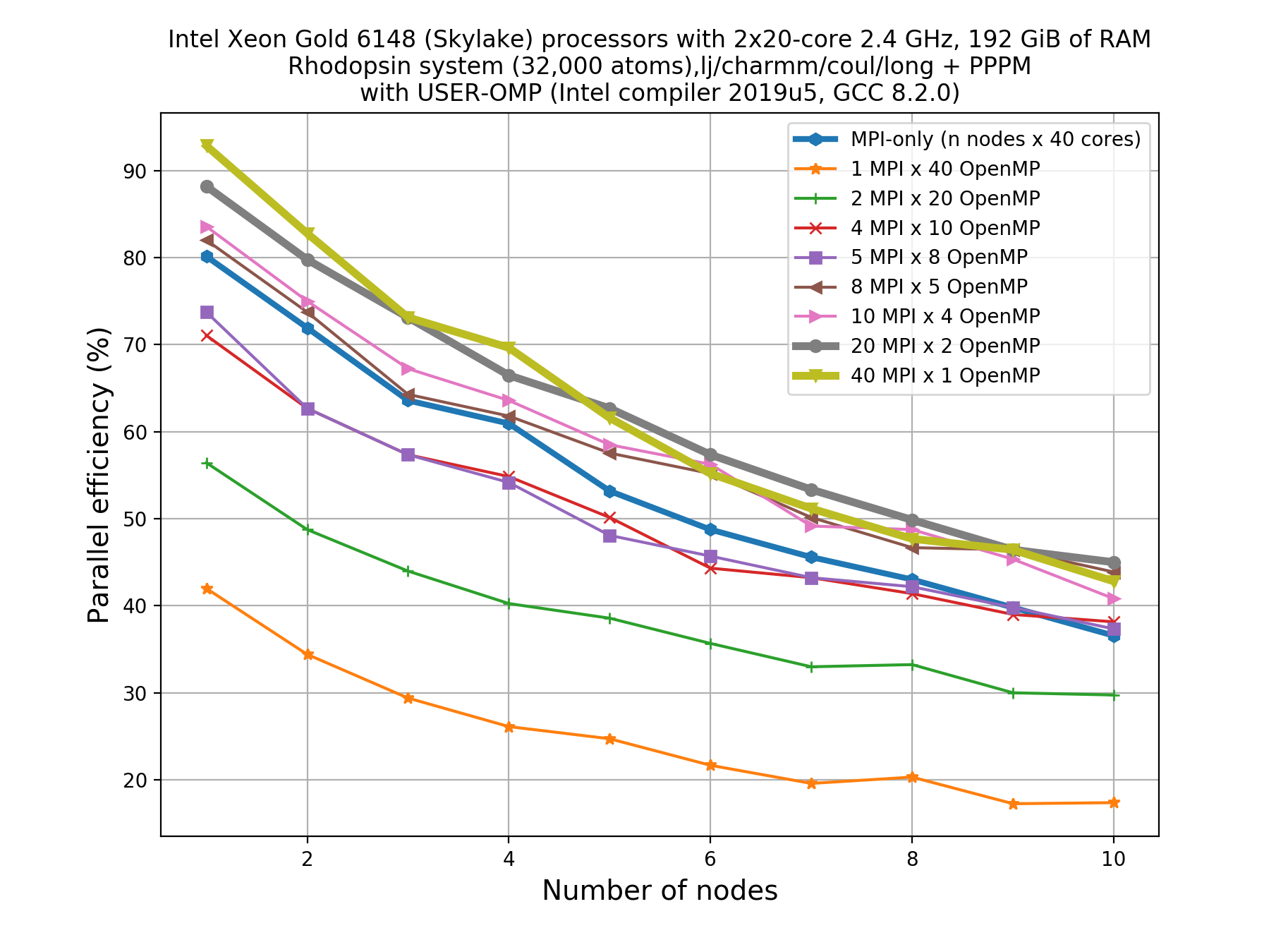
#!/bin/bash -x

# Ask for 1 nodes of resources for an MPI/OpenMP job for 5 minutes

#SBATCH --account=ecam
#SBATCH --nodes=1
#SBATCH --output=mpi-out.%j
#SBATCH --error=mpi-err.%j
#SBATCH --time=00:10:00

# Let's use the devel partition for faster queueing time since we have a tiny job.
# (For a more substantial job we should use --partition=batch)

#SBATCH --partition=devel

# Make sure that the multiplying the following 2 gives ncpus per node (24)

#SBATCH --ntasks-per-node=12
#SBATCH --cpus-per-task=2

# Prepare the execution environment
module purge
module use /usr/local/software/jureca/OtherStages
module load Stages/Devel-2019a
module load intel-para/2019a
module load LAMMPS/3Mar2020-Python-3.6.8-kokkos

# Also need to export the number of OpenMP threads so the application knows about it
export OMP_NUM_THREADS=$SLURM_CPUS_PER_TASK

# srun handles the MPI placement based on the choices in the job script file
srun lmp -in in.rhodo -sf omp -pk omp $OMP_NUM_THREADS
On a system of a node with 40 cores, if we want to see scaling, say up to 10 nodes, this means that a total of 80 calculations would need to be run since we have 8 MPI/OpenMP combinations for each node.
Thankfully, you don’t need to do the 80 calculations right now! Here’s an example plot for what that picture might look like:
Write down your observations based on this plot and make comments on any performance enhancement when you compare these results with the pure MPI runs.
Solution
For a system with 40 cores per node, the following combinations are possible:
- 1 MPI task with 40 OpenMP threads
- 2 MPI tasks with 20 OpenMP threads
- 4 MPI tasks with 10 OpenMP threads
- 5 MPI tasks with 8 OpenMP threads
- 8 MPI tasks with 5 OpenMP threads
- 10 MPI tasks with 4 OpenMP threads
- 20 MPI tasks with 2 OpenMP threads
- 40 MPI tasks with 1 OpenMP threads
For a perfectly scalable system, parallel efficiency should be equal to 100%, and as it approaches zero we say that the parallel performance is poor.
From the plot, we can make a few observations.
- As we increase number of nodes, the parallel efficiency decreases considerably for all the runs. This decrease in performance could be associated to the poor scalability of the
KspaceandNeighcomputations.- Parallel efficiency is increased by about 10-15% when we use mixed MPI+OpenMP approach even when we use only 1 OpenMP thread.
- The performance of hybrid runs are better than or comparable to pure MPI runs only when the number of OpenMP threads are less than or equals to five. This implies that USER-OMP package shows scalability only with lower numbers of threads.
Though we are seeing about 10-15% increase in parallel efficiency of hybrid MPI+OpenMP runs (using 2 threads) over pure MPI runs, still it is important to note that trends in loss of performance with increasing core number is similar in both of these types of runs thus indicating that this increase in performance might not be due to threading but rather due to other effects (like vectorisation).
In fact, there are overheads to making the kernels thread-safe. In LAMMPS, MPI-based parallelization almost always win over OpenMP until thousands of MPI ranks are being used where communication overheads become very significant.
How to invoke the GPU package
A question that you may be asking is how much speed-up would you expect from the GPU package. Unfortunately there is no easy answer for this. This can depend on many things starting from the hardware specification to the complexities involved with the specific problem that you are simulating. However, for a given problem one can always optimize the run-time parameters to extract the most out of a hardware. In the following section, we’ll discuss some of these tuning parameters for the simplest LJ-systems.
The primary aim for this following exercise is:
- To get a basic understanding of the various command line arguments that can control how a job is distributed among CPUs/GPUs, how to control CPU/GPU communications, etc.
- To get an initial idea on how to play with different run-time parameters to get an optimum performance.
- Finally, one can also make a fair comparison of performance between a regular LAMMPS run, the GPU package and a KOKKOS implementation of GPU functionality.
- Moreover, this exercise will also help the users to extend the knowledge of using the package command so that they can figure out by themselves how to use other accelerator packages in LAMMPS.
Before invoking the GPU package, you must ask the following questions:
- Do I have an access to a computing node with a GPU?
- Is my LAMMPS binary built with GPU package? HOW TO CHECK THIS?
If the answer to these two questions is a yes then we you can proceed to the following section.
Basic syntax: arguments and keywords
As discussed above, you need to use the package command to invoke the GPU package.
To use the GPU package for an accelerator you need to select gpu as <style>. Next
you need to choose proper <arguments> for the gpu style. The main argument for the
gpu style is:
ngpu: This sets the number of GPUs per node. There must be at least as many MPI tasks per node as GPUs. If there are more MPI tasks (per node) than GPUs, multiple MPI tasks will share each GPU (which may not be optimal).
In <arguments>, we can also have a number of keywords and their corresponding
values. These keyword/values provides you enhanced flexibility to distribute your
job among CPUs and GPUs in an optimum way. For a quick reference, the table below
could be useful.
Keywords of the GPU package
For more details, see the official documentation for LAMMPS.
Keywords Use Default value neighspecifies where neighbor lists for pair style computation will be built: GPU or CPU. yesnewtonsets the Newton flags for pairwise (not bonded) interactions to off or on. Only off value is supported with the GPU package currently (version 3Mar20)off(only)binsizesets the size of bins used to bin atoms in neighbor list builds performed on the GPU, if neigh = yes is set 0.0 splitused for load balancing force calculations between CPU and GPU cores in GPU-enabled pair styles 1.0(all on GPU),-1.0(dynamic load balancing), 0 <split<1.0 (custom)gpuIDallows selection of which GPUs on each node will be used for a simulation tpasets the number of GPU thread per atom used to perform force calculations. It is used for fining tuning of performance. When you use large cutoffs or do a simulation with a small number of particles per GPU, you may increase the value of this keyword to see if it can improve performance. The number of threads per atom must be chosen as a power of 2 and cannot be greater than 32 (version 3Mar20).1deviceused to tune parameters optimized for a specific accelerator and platform when using OpenCL blocksizeallows you to tweak the number of threads used per thread block minimum = 32
Not surprisingly, the syntax we use is similar to that of USER-OMP package:
srun lmp -in in.lj -sf gpu -pk gpu 2 neigh yes newton off split 1.0
Learn to call the GPU package from the command-line
Derive a command line to submit a LAMMPS job for the LJ system described by the following input file (
in.lj). Use command/package keywords from the table should to set the following conditions:
- Use 4 GPUs and a full node of MPI ranks
- Neighbour lists built on CPUs
- Dynamic load balancing between CPUs and GPUs
# 3d Lennard-Jones melt
variable        x index 60
variable        y index 60
variable        z index 60
variable        t index 500

variable        xx equal 1*$x
variable        yy equal 1*$y
variable        zz equal 1*$z

variable        interval equal $t/2

units           lj
atom_style      atomic

lattice         fcc 0.8442
region          box block 0 ${xx} 0 ${yy} 0 ${zz}
create_box      1 box
create_atoms    1 box
mass            1 1.0

velocity        all create 1.44 87287 loop geom

pair_style      lj/cut 2.5
pair_coeff      1 1 1.0 1.0 2.5

neighbor        0.3 bin
neigh_modify    delay 0 every 20 check no

fix             1 all nve

thermo          ${interval}
thermo_style custom step time  temp press pe ke etotal density
run             $t
Solution
srun lmp -in in.lj -sf gpu -pk gpu 2 neigh no newton off split -1.0The breakdown of the command is as follows;
-pk gpu 4- Setting GPU package and number of GPUs (2)-sf gpu- GPU package related fix/pair stylesneigh no- Anovalue ofneighkeyword indicates neighbour list built in the CPUsnewton off- Currently, only an off value is allowed as all GPU package pair styles require this setting.split -1.0- Dynamic load balancing option between CPUs and GPUs when value =-1NB: It is important to fix the number of MPI ranks in your submission script, and request the number of GPUs you wish to utilise. These will change depending on your system.
How to request and configure GPU resources is usually quite specific to the HPC system you have access to. Below you will find an example of how to submit the job we just constructed to JURECA.
#!/bin/bash -x

# Ask for 1 nodes of resources for an MPI/GPU job for 10 minutes

#SBATCH --account=ecam
#SBATCH --nodes=1
#SBATCH --output=mpi-out.%j
#SBATCH --error=mpi-err.%j
#SBATCH --time=00:10:00

# Configure the GPU usage (we request to use all 4 GPUs on a node)
#SBATCH --partition=develgpus
#SBATCH --gres=gpu:4

# Use this many MPI tasks per node (maximum 24)
#SBATCH --ntasks-per-node=24

module purge
module use /usr/local/software/jureca/OtherStages
module load Stages/Devel-2019a
module load intel-para/2019a
# Note we are loading a different LAMMPS package
module load LAMMPS/9Jan2020-cuda

srun lmp -in in.lj -sf gpu -pk gpu 4 neigh no newton off split -1.0
Understanding the GPU package output
At this stage, once you complete a job successfully, it is time to look for a few things in the LAMMPS output file. The first of these is to check that LAMMPS is doing the things that you asked for and the rest are to tell you about the performance outcome.
It prints about the device information both in the screen-output and the log file. You would notice something similar to;
-------------------------------------------------------------------------------
- Using acceleration for lj/cut:
-  with 12 proc(s) per device.
-  with 1 thread(s) per proc.
-------------------------------------------------------------------------------
Device 0: Tesla K80, 13 CUs, 10/11 GB, 0.82 GHZ (Double Precision)
Device 1: Tesla K80, 13 CUs, 0.82 GHZ (Double Precision)
-------------------------------------------------------------------------------

Initializing Device and compiling on process 0...Done.
Initializing Devices 0-1 on core 0...Done.
Initializing Devices 0-1 on core 1...Done.
Initializing Devices 0-1 on core 2...Done.
Initializing Devices 0-1 on core 3...Done.
Initializing Devices 0-1 on core 4...Done.
Initializing Devices 0-1 on core 5...Done.
Initializing Devices 0-1 on core 6...Done.
Initializing Devices 0-1 on core 7...Done.
Initializing Devices 0-1 on core 8...Done.
Initializing Devices 0-1 on core 9...Done.
Initializing Devices 0-1 on core 10...Done.
Initializing Devices 0-1 on core 11...Done.
The first thing that you should notice here is that it’s using an acceleration for the
pair potential lj/cut
and for this purpose it is using two devices (Device 0 and Device 1) and 12 MPI-processes per
device. That is what we asked for using 2 GPUs (-pk gpu 2) and in this case there
were 24 cores on the node. The number of tasks is shared equally by
each GPU. The detail about the graphics card is also printed, along
with the numerical precision used by the GPU package is also printed. In this case, it
is using double precision. Next it shows how many MPI-processes are spawned per GPU.
Accelerated version of pair-potential
This section of the output shows you that it is actually using the accelerated version of the
pair potential lj/cut. You can see that it is using lj/cut/gpu though in your input file you
mentioned this as pair_style lj/cut 2.5. This is what happens when you use the -sf gpu
command-line switch. This automatically ensures that the correct accelerated version is called for
this run.
(1) pair lj/cut/gpu, perpetual
    attributes: full, newton off
    pair build: full/bin/anomaly
    stencil: full/bin/3d
    bin: standard
Performance section
The following screen-output tells you all about the performance. Some of these terms are already
discussed in the previous episode.
When you use the
GPU package you see an extra block
of information known as Device Time Info (average). This gives you a breakdown of how
the devices (GPUs) have been utilised to do various parts of the job.
Loop time of 7.56141 on 24 procs for 500 steps with 864000 atoms

Performance: 28566.100 tau/day, 66.125 timesteps/s
95.3% CPU use with 24 MPI tasks x 1 OpenMP threads

MPI task timing breakdown:
Section |  min time  |  avg time  |  max time  |%varavg| %total
---------------------------------------------------------------
Pair    | 2.2045     | 2.3393     | 2.6251     |   6.1 | 30.94
Neigh   | 2.8258     | 2.8665     | 3.0548     |   2.9 | 37.91
Comm    | 1.6847     | 1.9257     | 2.0968     |   6.8 | 25.47
Output  | 0.0089157  | 0.028466   | 0.051726   |   6.7 |  0.38
Modify  | 0.26308    | 0.27673    | 0.29318    |   1.5 |  3.66
Other   |            | 0.1247     |            |       |  1.65

Nlocal:    36000 ave 36186 max 35815 min
Histogram: 1 2 3 4 2 3 3 4 1 1
Nghost:    21547.7 ave 21693 max 21370 min
Histogram: 1 1 0 5 5 2 4 1 2 3
Neighs:    0 ave 0 max 0 min
Histogram: 24 0 0 0 0 0 0 0 0 0
FullNghs:  2.69751e+06 ave 2.71766e+06 man 2.6776e+06 min
Histogram: 1 1 4 4 3 2 3 4 1 1

Total # of neighbors = 64740192
Ave neighs/atom = 74.9308
Neighbor list builds = 25
Dangerous builds not checked


---------------------------------------------------------------
      Device Time Info (average):
---------------------------------------------------------------
Data Transfer:   0.9243 s.
Data Cast/Pack:  0.6464 s.
Neighbor copy:   0.5009 s.
Neighbor unpack: 0.0000 s.
Force calc:      0.6509 s.
Device Overhead: 0.5445 s.
Average split:   0.9960.
Threads / atom:  4.
Max Mem / Proc:  53.12 MB.
CPU Driver_Time: 0.5243 s.
CPU Idle_Time:   0.9986 s.
---------------------------------------------------------------


Please see the log.cite file for references relevant to this simulation

Total wall time: 0:00:15
Choosing your parameters
You should now have an idea of how to submit a LAMMPS job that uses the GPU package as an accelerator. Optimizing the run may not be that straight-forward however. You can have numerous possibilities of choosing the argument and the keywords. Not only that, the host CPU might have multiple cores. More choices would arise from here.
As a rule of thumb, you must have at least same number of MPI processes as the number of GPUs available to you. But often, using many MPI tasks per GPU gives you the better performance. As an example, if you have 4 physical GPUs, you must initiate (at least) 4 MPI processes for this job. Let’s assume that you have a CPU with 12 cores. This gives you flexibility to use at most 12 MPI processes and the possible combinations are 4 GPUs with 4 CPUs, 4 GPUs with 8 CPUs and 4 GPUs with 12 CPUs. Though it may sound like that 4 GPUs with 12 CPUs will provide the maximum speed-up, that may not be the case! This entirely depends on the problem and also on other settings which can in general be controlled by the keywords mentioned in the above table. Moreover, one may find that for a particular problem using 2 GPUs instead of 4 GPUs may give better performance, and this is why it is advisable to figure out the best possible set of run-time parameters by following a thorough optimization before starting the production runs. This might save you a lot of resources and time!
Case study
Let’s look at the result of doing such a study for a node with 4 GPUs and 24 CPU cores. We set
t = 5000and use 3 sets of values for our volume:
x = y = z = 10= 4,000 atomsx = y = z = 40= 256,000 atomsx = y = z = 140= 11,000,000 atomsWe choose package keywords such that neighbour list building and force computations are done entirely on the GPUs:
-sf gpu -pk gpu 4 neigh yes newton off split 1.0where 4 GPUs are being used.
On a system with 2x12 cores per node and four GPUs, the different combinations are;
- 4 GPUs/4 MPI tasks
- 4 GPUs/8 MPI tasks
- 4 GPUs/12 MPI tasks
- 4 GPUs/16 MPI tasks
- 4 GPUs/20 MPI tasks
- 4 GPUs/24 MPI tasks
Across all GPU/MPI combinations and system sizes (4K, 256K, 11M), there are a total of 18 runs. The final plot is shown below.
What observations can you make about this plot?
Solution
The main observations you can take from this are:
- For the system with 4000 atoms, increasing the number of MPI tasks actually degrades the overall performance.
- For the 256K system, we can notice an initial speed-up with increasing MPI task counts up to 4 MPI ranks per GPU, and then it starts declining again.
- For the largest 11M atom system, there is a sharp increase of speed-up up to 4 MPI ranks per GPU, and then also a relatively slow but steady increase is seen with increasing MPI tasks per GPU (in this case, 6 MPI tasks per GPU).
Possible explanation:
- For the smallest system, the number of atoms assigned to each GPU or MPI ranks is very low. The system size is so small that considering GPU acceleration is practically meaningless. In this case you are employing far too many workers to complete a small job and therefore it is not surprising that the scaling deteriorates with increasing MPI tasks. In fact, you may try to use 1 GPU and a few MPI task to see if the performance increases in this case.
- As the system size increases, the normalized speed-up factor per node increases with increasing MPI tasks per GPU since in these cases the MPI tasks are busy in computing rather than spending time in communicating each other, i.e. computational overhead exceeds the communication overheads.
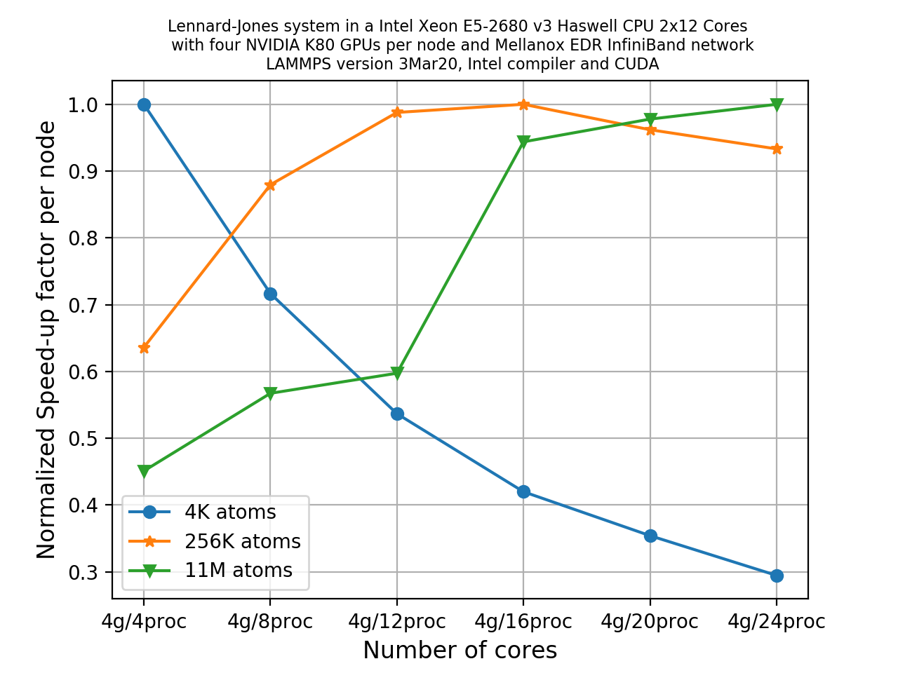
Load balancing: revisited
We have discussed load balancing in the previous episode due to the potential for under-performance
in systems with an inhomogeneous distribution of particles. We discussed earlier that it can be
done using the split keyword. Using this keyword a fixed fraction of particles is offloaded to
the GPU while force calculation for the other particles occurs simultaneously on the CPU. When you
set split = 1 you are offloading entire force computations to the GPUs (discussed in previous
exercise). What fraction of particles would be offloaded to GPUs can be set explicitly by choosing
a value ranging from 0 to 1. When you set its value to -1, you are switching on dynamic load
balancing. This means that LAMMPS selects the split factor dynamically.
Switching on dynamic load balancing
If we repeat the previous exercise but this time use dynamic load balancing (by changing the value of
splitto-1.0). We can see how the plot has changed significantly due to dynamic load balancing increasing the performance.
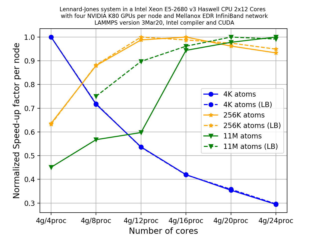
CPU versus GPU
By now we have idea about some of the ‘preferred’ tuning parameters for an LJ-system. For the current exercise, let us take the system with ~11 million atoms, i.e.
x = y = z = 140andt = 500and for this size of atoms, we know from our previous example thatA GPUs/B MPItasks (whereAis number of GPUs andBis number of cores in a node) gives the best performance. We wish to see how much acceleration a GPU package can provide if we offload the entire force computation and neighbour list building to the GPUs. This can be done using;-sf gpu -pk gpu 4 neigh yes newton off split 1.0The plot below shows an HPC system with 2x12 CPU cores per node and 2 GPUs (4 visible devices) per node. Two sets of runs (i.e. with and without the GPU package) were executed with up to 8 nodes. Performance data was extracted from the log files in the unit of
timesteps/s, and speed-up factors were calculated for each node.
We can see a reasonable acceleration when we use the GPU package for all the runs consistently. The calculated speed-up factors show that we obtain maximum speed-up (~5.2x) when we use 1 node, then it gradually decreases (for 2 nodes it is 5x) and finally saturates to a value of ~4.25x when we run using 3 nodes or higher (up to 8 nodes is tested here).
The slight decrease in speed-up with increasing number of nodes could be related to the inter-node communications. But overall the GPU package offers quite a fair amount of performance enhancement over the regular CPU version of LAMMPS with MPI parallelization.
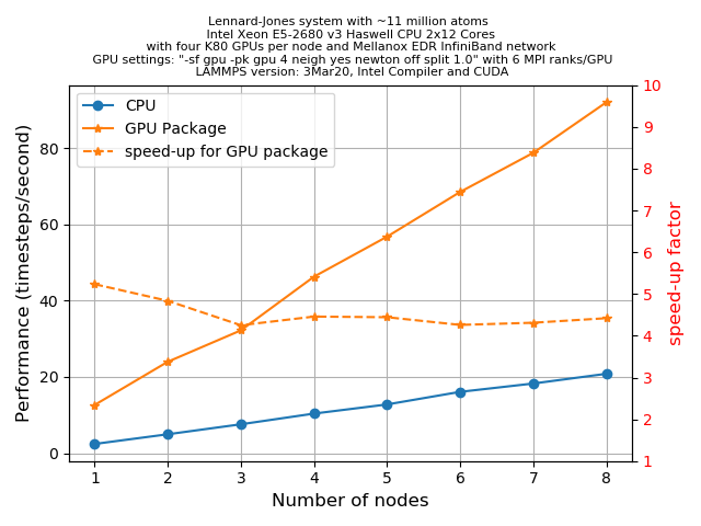
Key Points
The five accelerator packages currently offered by LAMMPS are i) OPT, ii) USER-INTEL, iii) USER-OMP, iv) GPU, v) KOKKOS
KOKKOS is available for use on all types of hardware. Other accelerator packages are hardware specific
To invoke a package in LAMMPS, the notation is
package <style> <arguments>, wherestyleis the package you want to invoke
Invoking KOKKOS
Overview
Teaching: 25 min
Exercises: 5 minQuestions
Why should I use KOKKOS?
How do I invoke KOKKOS within LAMMPS?
Objectives
Learn how to invoke KOKKOS in a LAMMPS run
Learn how to transition from a normal LAMMPS call to an accelerated call
KOKKOS
In recent times, the HPC industry has witnessed dramatic architectural revolution. Modern HPC architecture not only includes the conventional multi-core CPUs, but also many-core systems (GPUs are a good example of this but there are other technologies), and we don’t know yet where this revolution will end up! With the availability of so many cores for computing, one would naturally expect a ‘scalable’ speedup in performance. However, this scalability does not come without a cost: it may require several man-years to modify an existing code to make it compatible with (and efficient on) new hardware architectures.
Why do we need to modify a code for new architectures? This is because innovative hardware is usually designed with different/innovative philosophies of parallelization in mind, and these philosophies continue to develop to enhance performance. We frequently now need to use novel parallelization approaches other than (or as well as) the classic MPI-based approach to use the latest hardware. For example, on a shared memory platform one can use OpenMP (not so new), or, on a mixed CPU+GPU platform, one can use CUDA or OpenACC to parallelize your codes. The major issue with all these approaches is the performance portability which arises due to differences in hardware, and software implementations for hardware (writing CUDA code for NVIDIA GPUs won’t help you with Intel Xeon Phi). So, the question arises: Is there any way to ease this difficulty?
KOKKOS is one of the programming models that strives to be an answer to this portability issue. The primary objective of KOKKOS is to maximize the amount of user code that can be compiled for various devices but obtaining comparable performance as compared to if the code was written in a native language specific to that particular device. How does KOKKOS achieve this goal?
- It maps a C++ kernel to different backend languages (like CUDA and OpenMP for example).
- It also provides data abstractions to adjust (at compile time) the memory layout of data structures like 2D and 3D arrays to optimize performance on different hardware (e.g., GPUs prefer an opposite data layout to CPUs).
KOKKOS: A developing library
Why should we bother to learn about using KOKKOS?
The primary reason for KOKKOS being used by LAMMPS is that it allows you to write a single pair style in C++ without (much) understanding of GPU programming, that will then work on both GPUs (or Xeon Phi or another supported hardware) and CPUs with or without multi-threading.
It cannot (currently) fully reach the performance of the USER-INTEL or the GPU packages on particular CPUs and GPUs, but adding new code for a pair style, for which something similar already exists, is significantly less effort with KOKKOS and requires significantly less programming expertise in vectorization and directive based SIMD programming or CPU computing. Also support for a new kind of computing hardware will primarily need additional code in the KOKKOS library and just a small amount of programming setup/management in LAMMPS.
What is the KOKKOS package in LAMMPS?
The KOKKOS package in LAMMPS is implemented to gain performance without losing portability. Various pair styles, fixes and atom styles have been updated in LAMMPS to use the data structures and macros as provided by the KOKKOS C++ library so that when LAMMPS is built with KOKKOS features enabled targeting the hardware available on the HPC resource, it can provide good performance for that hardware when all the runtime parameters are chosen sensibly. What are the things that it currently supports?
- It can be run on multi-core CPUs, many-core CPUS, NVIDIA GPUs and and Intel Phis.
- It provides three modes of execution: Serial (MPI-only for CPUs and Phi), OpenMP (via
threading for many-core CPUs and Phi), and CUDA (for NVIDIA GPUs)
- It is currently designed for one-to-one CPU to GPU ratio
- Care has been taken to minimize performance overhead due to CPU-GPU communication. This can be achieved by ensuring that most of the codes can be run on GPUs once assigned by the CPU and when all the jobs are done, it is communicated back to CPU, thus minimising the amount of data transfer between CPU and GPU.
- It provides reasonable scalability to many OpenMP threads.
- Currently supports double precision only (as of July 2020, but mixed precision is under development).
- It is under heavy development and adoption by LAMMPS, so more features and flexibilities are expected in future versions of LAMMPS.
The list of LAMMPS features that is supported by KOKKOS (as of July 2020) is given below:
| Atom Styles | Pair Styles | Fix Styles | Compute Style | Bond Styles | Angle Styles | Dihedral Styles | Improper Styles | K-space Styles |
|---|---|---|---|---|---|---|---|---|
| Angle | Buck/coul/cut | Deform | Temp | Fene | Charm | Charm | Harmonic | Pppm |
| Atomic | Buck/coul/long | Langevin | Harmonic | Harmonic | Opls | |||
| Bond | Etc. | Momentum | ||||||
| Charge | Etc. | Nph | ||||||
| Full | Npt | |||||||
| Molecular | Nve | |||||||
| Nvt | ||||||||
| Qeq/Relax | ||||||||
| Reaxc/bonds | ||||||||
| Reaxc/species | ||||||||
| Setforce | ||||||||
| Wall/reflect |
This list is likely to be subject to significant changes over time as newer versions of KOKKOS are released.
How to invoke KOKKOS package in a LAMMPS run?
In the previous episode you learned how to call an accelerator package in LAMMPS. The basic syntax of this command is;
package <style> <arguments>
where <arguments> can potentially include a number of keywords and their corresponding
values.
In this case, you will need to use kokkos as <style> with suitable arguments/keywords.
For KOKKOS these keyword/values provides you enhanced flexibility to distribute your job among CPUs and GPUs in an optimum way. As a quick reference, the following table could be useful:
Guide to KOKKOS keywords/values
Keywords what it does? Default value neighThis keyword determines how a neighbour list is built. Possible values are half,fullfullfor GPUs andhalffor CPUsneigh/qeqneigh/threadnewtonsets the Newton flags for pairwise and bonded interactions to off or on offfor GPU andonfor CPUbinsizesets the size of bins used to bin atoms in neighbor list builds 0.0for CPU. On GPUs, the default is twice the CPU valuecommIt determines whether the CPU or GPU performs the packing and unpacking of data when communicating per-atom data between processors. Values could be no,hostordevice.nomeans pack/unpack will be done in non-KOKKOS modecomm/exchangeThis defines ‘exchange’ communication which happens only when neighbour lists are rebuilt. Values could be no,hostordevicecomm/forwardThis defines forward communication and it occurs at every timestep. Values could be no,hostordevicecomm/reverseIf the newtonoption is set toon, this occurs at every timestep. Values could beno,hostordevicecuda/awareThis keyword is used to choose whether CUDA-aware MPI will be used. In cases where CUDA-aware MPI is not available, you must explicitly set it to offvalue otherwise it will result in an error.offRules of thumb
neigh: When you usefulllist, all the neighbors of atomiare stored with atomi. On the contrary, for ahalflist, thei-jinteraction is stored either with atomiorjbut not both. For the GPU, a value offullforneighkeyword is often more efficient, and in case of CPU a value ofhalfis often faster.newton: Using this keyword you can turn Newton’s 3rd lawonorofffor pairwise and bonded interactions. Turning thisonmeans less computation and more communication, and setting itoffmeans interactions will be calculated by both processors if these interacting atoms are being handled by these two different processors. This results in more computation and less communication. Definitely for GPUs, less communication is usually the better situation. Therefore, a value ofofffor GPUs is efficient while a value ofoncould be faster for CPUs.binsize: Default value is given in the above table. But there could be exceptions. For example, if you use a larger cutoff for the pairwise potential than the normal, you need to override the default value ofbinsizewith a smaller value.comm,comm/exchange,comm/forward,comm/reverse: From the table you can already tell what it does. Three possible values areno,hostanddevice. For GPUs,deviceis faster if all the styles used in your calculation are KOKKOS-enabled. But, if not, it may results in communication overhead due to CPU-GPU communication. For CPU-only systems,hostis the fastest. For Xeon Phi and CPU-only systems,hostanddevicework identically.cuda/aware: When we use regular MPI, multiple instances of an application is launched and distributed to many nodes in a cluster using the MPI application launcher. This passes pointers to host memory to MPI calls. But, when we want to use CUDA and MPI together, it is often required to send data from the GPU instead of the CPU. CUDA-aware MPI allows the GPU data to pass directly through MPI send/receive calls without first which copying the data from device to host, and thus CUDA-aware MPI helps to eliminate the overhead due to this copying process. However, not all HPC systems have the CUDA-aware MPI available and it results in aSegmentation Faulterror at runtime. We can avoid this error by setting its value tooff(i.e.cuda/aware off). Whenever a CUDA-aware MPI is available to you, you should not need to use this (the default should be faster).
Invoking KOKKOS through input file or through command-line?
Unlike the USER-OMP or the GPU package in the previous episode which supports either OpenMP or GPU, the KOKKOS package supports both OpenMP and GPUs. This adds additional complexity to the command-line to invoke appropriate execution mode (OpenMP or GPU) when you decide to use KOKKOS for your LAMMPS runs. In the following section, we’ll touch on a few general command-line features which are needed to call KOKKOS. More detailed OpenMP or GPU specific command-line switches will be discussed in later episodes.
Let us recall the command-line to submit a LAMMPS job that uses USER-OMP as an accelerator package (see here to refresh your memory).
srun lmp -in in.lj -sf omp -pk omp $OMP_NUM_THREADS neigh no
We can perform a straight-forward to edit the above command-line to try to make it appropriate for a KOKKOS run. A few points to keep in mind:
- To enable KOKKOS package you need to use a switch
-k on. - To use KOKKOS enabled styles (pair styles/fixes etc.), you need one additional
switch
-sf kk. This will append the/kksuffix to all the styles that KOKKOS supports in LAMMPS. For example, when you use this, thelj/charmm/coul/longpair style would be read aslj/charmm/coul/long/kkat runtime.
With these points in mind, the above command-line could be modified to start making it ready for KOKKOS:
srun lmp -in in.lj -k on -sf kk
But, unfortunately, this above command-line is still incomplete. We have not yet passed any
information about the package <arguments> yet. These might include information about
the execution mode (OpenMP or GPU), or the number of OpenMP threads,
or the number of GPUs that we want to use for this run, or any other keywords (and
values). We’ll discuss more about them in the following episodes.
Key Points
KOKKOS is a templated C++ library which allows a single implementation of a software application on different kinds of hardware
KOKKOS with OpenMP
Overview
Teaching: 30 min
Exercises: 15 minQuestions
How do I utilise KOKKOS with OpenMP
Objectives
Utilise OpenMP and KOKKOS on specific hardware
Be able to perform a scalability study on optimum command line settings
Using OpenMP threading through the KOKKOS package
In this episode, we’ll be learning to use KOKKOS package with OpenMP execution for multi-core CPUs. First we’ll get familiarized with the command-line options to run a KOKKOS OpenMP job in LAMMPS. This will be followed by a case study to gain some hands-on experience to use this package. For the hands-on part, we’ll take the same rhodopsin system which we have used previously as a case study. We shall use the same input file and repeat similar scalability studies for the mixed MPI/OpenMP settings as we did it for the USER-OMP package.
Factors that can impact performance
- Know your hardware: get the number of physical cores per node available to you. Take care such that
(number of MPI tasks) * (OpenMP threads per task) <= (total number of physical cores per node)- Check for hyperthreading: Sometimes a CPU splits its each physical cores into multiple virtual cores. Intel’s term for this is hyperthreads (HT). When hyperthreading is enabled, each physical core appears as (usually) two logical CPU units to the OS and thus allows these logical cores to share the physical execution space. This may result in a ‘slight’ performance gain. So, a node with 24 physical cores appears as 48 logical cores to the OS if HT is enabled. In this case,
(number of MPI tasks) * (OpenMP threads per task) <= (total number of virtual cores per node)- CPU affinity: CPU affinity decides whether a thread running on a particular core is allowed to migrate to another core (if the operating system thinks that is a good idea). You can set CPU affinity masks to limit the set of cores that the thread can migrate to, for example you usually do not want your thread to migrate to another socket since that could mean that it is far away from the data it needs to process and could introduce a lot of delay in fetching and writing data.
- Setting OpenMP Environment variables:
OMP_NUM_THREADS,OMP_PROC_BIND,OMP_PLACESare the ones we will touch here:
OMP_NUM_THREADS: sets the number of threads to use for parallel regionsOMP_PROC_BIND: set the thread affinity policy to be used for parallel regionsOMP_PLACES: specifies on which CPUs (or subset of cores of a CPU) the threads should be placed
Command-line options to submit a KOKKOS OpenMP job in LAMMPS
In this episode, we’ll learn to use KOKKOS package with OpenMP for multi-core CPUs. To run the KOKKOS package, the following three command-line switches are very important:
-k on: This enables KOKKOS at runtime-sf kk: This appends the “/kk” suffix to KOKKOS-supported LAMMPS styles-pk kokkos: This is used to modify the default package KOKKOS options
To invoke the OpenMP execution mode with KOKKOS, the -k on switch takes additional
arguments for hardware settings as shown below:
-k on t Nt: Using this switch you can specify the number of OpenMP threads,Nt, that you want to use per node. You should also set a proper value for your OpenMP environment variables. You can do this withexport OMP_NUM_THREADS=4if you like to use 4 threads per node (
Ntis 4). Using this environment variable allows you to use-k on t $OMP_NUM_THREADSon the command line or in your job scripts.You should also set some other environment variables to help with thread placement. Good default options with OpenMP 4.0 or later are:
export OMP_PROC_BIND=spread
export OMP_PLACES=threads
Get the full command-line
Try to create a job script to submit a LAMMPS job for the rhodopsin case study) such that it invokes KOKKOS with OpenMP threading to accelerate the job using 2 nodes, 2 MPI ranks per node with half the available cores on a node used as OpenMP threads per rank, and the default package options.
Solution
#!/bin/bash -x

# Ask for 1 nodes of resources for an MPI/OpenMP job for 5 minutes

#SBATCH --account=ecam
#SBATCH --nodes=1
#SBATCH --output=mpi-out.%j
#SBATCH --error=mpi-err.%j
#SBATCH --time=00:10:00

# Let's use the devel partition for faster queueing time since we have a tiny job.
# (For a more substantial job we should use --partition=batch)

#SBATCH --partition=devel

# Make sure that the multiplying the following 2 gives ncpus per node (24)

#SBATCH --ntasks-per-node=2
#SBATCH --cpus-per-task=12

# Prepare the execution environment
module purge
module use /usr/local/software/jureca/OtherStages
module load Stages/Devel-2019a
module load intel-para/2019a
module load LAMMPS/3Mar2020-Python-3.6.8-kokkos

# Also need to export the number of OpenMP threads so the application knows about it
export OMP_NUM_THREADS=$SLURM_CPUS_PER_TASK
# Set some pinning hints as well
export OMP_PROC_BIND=spread
export OMP_PLACES=threads

# srun handles the MPI task placement and affinities based on the choices in the job script file
srun lmp -in in.rhodo -k on t $OMP_NUM_THREADS -sf kk
A solution including affinity using the OpenMPI MPI would include runtime binding mechanisms like
--bind-to socketand--map-by socketwhich ensures that OpenMP threads cannot move between sockets (but how something like this is done is dependent on the MPI runtime used).OMP_PROC_BINDandOMP_PLACESwould then influence what happens to the OpenMP threads on each socket.
Finding out optimum command-line settings for the package command
There is some more work to do before we can jump into a thorough scalability study when
we use OpenMP in KOKKOS which comes with a few extra package arguments and
corresponding keywords (see the
previous episode for
a list of all options) as compared to that offered by the USER-OMP package. These
are neigh, newton, comm and binsize. The first thing that we need to do here is to
find what values of these keywords offer the fastest runs. Once we know the optimum
settings, we can use them for all the runs needed to perform the scalability studies.
In the last exercise, we constructed a command-line example to submit a LAMMPS job with
the default
package setting for the KOKKOS OpenMP run. But, often the default package setting
may not provide the fastest runs. Before jumping to production runs, we should investigate
other settings for these values to avoid wastage of our time and valuable
computing resources. In the next section, we’ll be showing how to do this with
rhodopsin example. An example of a set of command line arguments which shows
how these package related keywords can be invoked in your LAMMPS run would be
-pk kokkos neigh half newton on comm no.
The optimum values of the keywords
Using the rhodopsin input files (
in.rhodoanddata.rhodoas provided in the rhodopsin case study), run LAMMPS jobs for 1 OpenMP thread on 1 node using the following two set of parameters for thepackagecommand:
neigh full newton off comm noneigh half newton on neigh half comm host
What is the influence of
comm? What is implied in the output file?What difference does switching the values of
newton/neighhave? Why?Results obtained from a 40 core system
For a HPC setup which has 40 cores per node, the runtimes for all the MPI/OpenMP combinations and combination of keywords is given below:
neigh newton comm binsize 1MPI/40t 2MPI/40t 4MPI/10t 5MPI/8t 8MPI/5t 10MPI/4t 20MPI/2t 40MPI/1t full off no default 172 139 123 125 120 117 116 118 full off host default 172 139 123 125 120 117 116 118 full off dev default 172 139 123 125 120 117 116 119 full on no default 176 145 125 128 120 119 116 118 half on no default 190 135 112 119 103 102 97 94
The influence on
commcan be seen in the output file, as it prints the following;WARNING: Fixes cannot yet send data in KOKKOS communication, switching to classic communication (src/KOKKOS/comm_kokkos.cpp:493)This means the fixes that we are using in this calculation are not yet supported in KOKKOS communication and hence using different values of the
commkeyword makes no difference.Switching on
newtonand usinghalfneighbour list make the runs faster for most of the MPI/OpenMP settings. Whenhalfneighbour list and OpenMP is being used together in KOKKOS, it uses data duplication to make it thread-safe. When you use relatively few numbers of threads (8 or less) this could be fastest and for more threads it becomes memory-bound (since there are more copies of the same data filling up RAM) and suffers from poor scalability with increasing thread-counts. If you look at the data in the above table carefully, you will notice that using 40 OpenMP threads forneigh=halfandnewton=onmakes the run slower. On the other hand, when you use only 1 OpenMP thread per MPI rank, it requires no data duplication or atomic operations, hence it produces the fastest run.So, we’ll be using
neigh half newton on comm hostfor all the runs in the scalability study below.
Rhodopsin scalability study with KOKKOS
Doing a scalability study would be a time consuming undertaking, a full study would again require a total of 80 calculations for 10 nodes. Below is the result of such a study on an available system (FIX SCALES)
Compare this plot with the plot given in a previous exercise. Write down your observations and make comments on any performance “enhancement” when you compare these results with the pure MPI runs.
Solution
Data for the pure MPI-based run is plotted with the thick blue line. Strikingly, none of the KOKKOS based MPI/OpenMP mixed runs show comparable parallel performance with the pure MPI-based approach. The difference in parallel efficiency is more pronounced for less node counts and this gap in performance reduces slowly as we increase the number of nodes to run the job. This indicates that to see comparable performance with the pure MPI-based runs we need to increase the number of nodes far beyond than what is used in the current study.
If we now compare the performance of KOKKOS OpenMP with the threading implemented with the USER-OMP package, there is quite a bit of difference.
This difference could be due to vectorization. Currently (version
7Aug19or3Mar20) the KOKKOS package in LAMMPS doesn’t vectorize well as compared to the vectorization implemented in the USER-OMP package. USER-INTEL should be even better than USER-OMP at vectorizing if the styles are supported in that package.The ‘deceleration’ is probably due to KOKKOS and OpenMP overheads to make the kernels thread-safe.
If we just compare the performance among the KOKKOS OpenMP runs, we see that parallel efficiency values are converging even for more thread-counts (1 to 20) as we increase the number of nodes. This is indicative that KOKKOS OpenMP scales better with increasing thread counts as compared to the USER-OMP package.
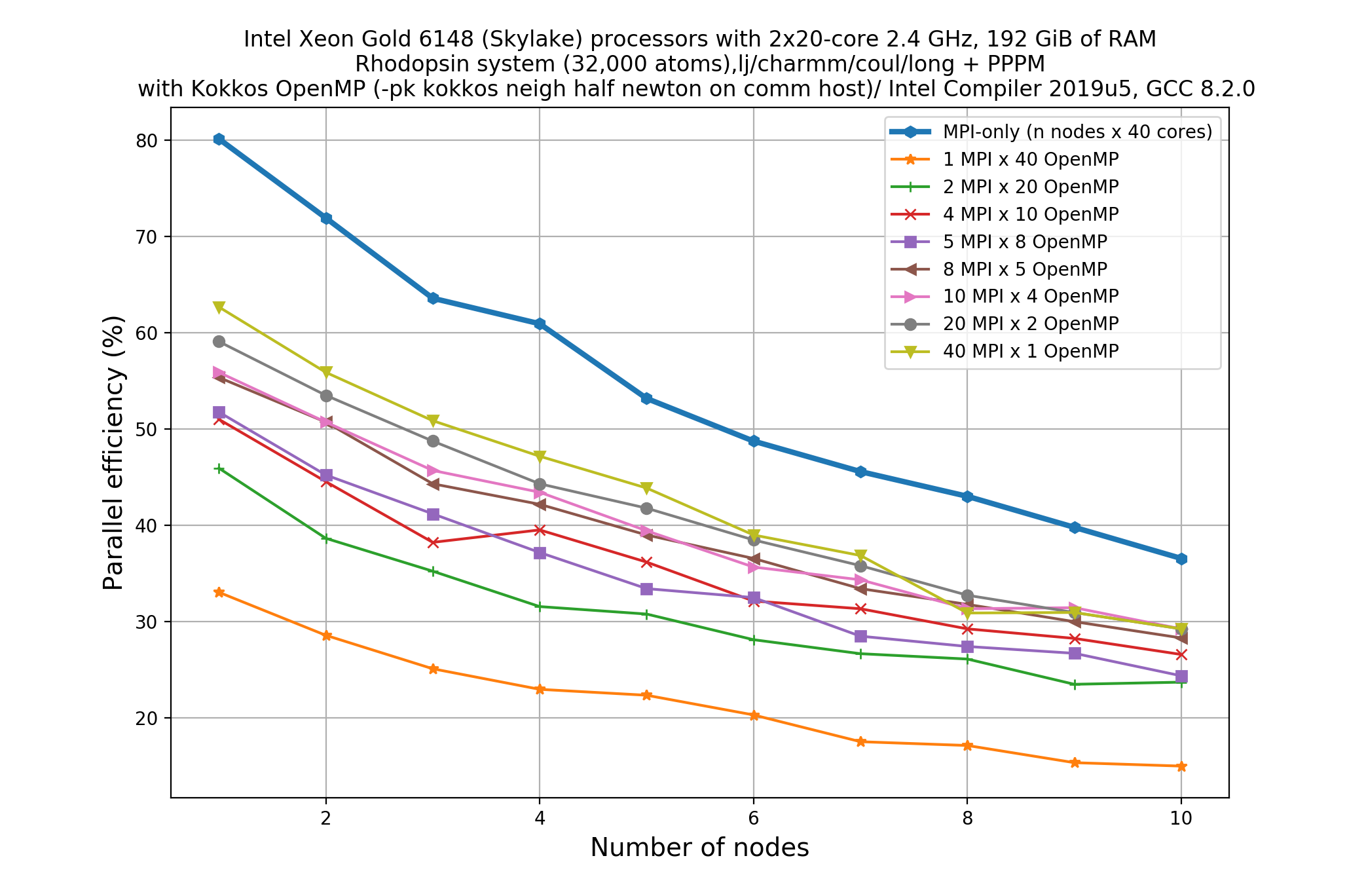
Key Points
The three command line switches,
-k on,-sf kkand-pk kokkosare needed to run the KOKKOS packageDifferent values of the keywords
neigh,newton,commandbinsizeresult in different runtimes
KOKKOS with GPUs
Overview
Teaching: 15 min
Exercises: 15 minQuestions
How do I use KOKKOS together with a GPU?
Objectives
What is the performance like?
Using GPU acceleration through the KOKKOS package
In this episode, we shall learn to how to use GPU acceleration using the KOKKOS
package in LAMMPS. In a
previous episode, we
have learnt the basic syntax of the package command that
is used to invoke the KOKKOS package in a LAMMPS run. The main arguments and the
corresponding keywords were discussed briefly in that chapter. In this episode, we shall
do practical exercises to get further hands-on experiences on using those commands.
Command-line options to submit a KOKKOS GPU job in LAMMPS
In this episode, we’ll learn to use KOKKOS package with GPUs. As we have seen, to run the KOKKOS package the following three command-line switches are very important:
-k on: This enables KOKKOS at runtime-sf kk: This appends the “/kk” suffix to KOKKOS-supported LAMMPS styles-pk kokkos: This is used to modify the default package KOKKOS options
To invoke the GPU execution mode with KOKKOS, the -k on switch takes additional
arguments for hardware settings as shown below:
-k on g Ngpu: Using this switch you can specify the number of GPU devices,Ngpu, that you want to use per node.
Before you start
- Know your host: get the number of physical cores per node available to you.
- Know your device: know how many GPUs are available on your system and know how to ask for them from your resource manager (SLURM, etc.)
- CUDA-aware MPI: Check if you can use a CUDA-aware MPI runtime with your LAMMPS executable. If not then you will need to add
cuda/aware offto your<arguments>.
Creating a KOKKOS GPU job script
Create a job script to submit a LAMMPS job for the LJ system that you studied for the GPU package such that it invokes the KOKKOS GPU to
- accelerate the job using 1 node,
- uses all available GPU devices on the node,
- use the same amount of MPI ranks per node as there are GPUs, and
- uses the default package options.
Solution
#!/bin/bash -x

# Ask for 1 nodes of resources for an MPI/GPU job for 5 minutes

#SBATCH --account=ecam
#SBATCH --nodes=1
#SBATCH --output=mpi-out.%j
#SBATCH --error=mpi-err.%j
#SBATCH --time=00:10:00

# Configure the GPU usage (we request to use all 4 GPUs on a node)
#SBATCH --partition=develgpus
#SBATCH --gres=gpu:4

# Use this many MPI tasks per node (maximum 24)
#SBATCH --ntasks-per-node=4
#SBATCH --cpus-per-task=6

export OMP_NUM_THREADS=$SLURM_CPUS_PER_TASK
export OMP_PROC_BIND=spread
export OMP_PLACES=threads

module purge
module use /usr/local/software/jureca/OtherStages
module load Stages/Devel-2019a
module load intel-para/2019a
# Note we are loading a different LAMMPS package
module load LAMMPS/3Mar2020-gpukokkos

srun lmp -in in.lj -k on g 4 -sf kk -pk kokkos cuda/aware off
If you run it how does the execution time compare to the times you have seen for the GPU package?
A few tips on gaining speedup from KOKKOS/GPU
This information is collected from the LAMMPS website
- Hardware comptibility: For better performance, you must use Kepler or later generations of GPUs.
- MPI tasks per GPU: You should use one MPI task per GPU because KOKKOS tries to run everything on the GPU, including the integrator and other fixes/computes. One may get better performance by assigning multiple MPI tasks per GPU if some styles used in the input script have not yet been KOKKOS-enabled.
- CUDA-aware MPI library: Using this can provide significant performance gain. If this is not available, set it
offusing the-pk kokkos cuda/aware offswitch.neighandnewton: For KOKKOS/GPU, the default isneigh = fullandnewton = off. For Maxwell and Kepler generations of GPUs, the default settings are typically the best. For Pascal generations, settingneigh = halfandnewton = onmight produce faster runs.- binsize: For many pair styles, setting the value of
binsizeto twice that used for the CPU styles could offer speedup (and this is the default for the KOKKOS/GPU style)- Avoid mixing KOKKOS and non-KOKKOS styles: In the LAMMPS input file, if you use styles that are not ported to use KOKKOS, you may experience a significant loss in performance. This performance penalty occurs because it causes the data to be copied back and forth from the CPU repeatedly.
In the following discussion, we’ll work on a few exercises to get familiarized on some of these aspects (to some extent).
Exercise: Performance penalty due to use of mixed styles
- First, let us take the input and job script for the LJ-system in the last exercise. Make a copy of the job script that uses the following additional settings for KOKKOS:
newton offneigh fullcomm deviceUse the number of MPI tasks that equals to the number of devices. Measure the performance of of this run in
timesteps/s.- Make a copy of the LJ-input file called
in.mod.ljand replace the line near the end of the file:thermo_style custom step time temp press pe ke etotal densitywith
compute 1 all coord/atom cutoff 2.5 compute 2 all reduce sum c_1 variable acn equal c_2/atoms thermo_style custom step time temp press pe ke etotal density v_acn- Using the same KOKKOS setting as before, and the identical number of GPU and MPI tasks as previously, run the job script using the new input file. Measure the performance of this run in
timesteps/sand compare the performance of these two runs. Comment on your observations.Solution
Taking an example from a HPC system with 2x12 cores per node and 4 GPUs, using 1 MPI task per GPU, the following was observed.
First, we ran with
in.lj. Second, we modified this input as mentioned above (to becomein.mod.lj) and performance for both of these runs are measured in units oftimesteps/s. We can get this information from the log/screen output files. The comparison of performance is given in this table:
Input Performance (timesteps/sec) Performance loss in.lj(all KOKKOS enabled styles used)8.097 in.mod.lj(non-KOKKOS style used:compute coord/atom)3.022 2.68 In
in.mod.ljwe have used styles that are not yet ported to KOKKOS. We can check this from the log/screen output files:(1) pair lj/cut/kk, perpetual attributes: full, newton off, kokkos_device pair build: full/bin/kk/device stencil: full/bin/3d bin: kk/device (2) compute coord/atom, occasional attributes: full, newton off pair build: full/bin/atomonly stencil: full/bin/3d bin: standardIn this case, the pair style is KOKKOS-enabled (
pair lj/cut/kk) while the compute stylecompute coord/atomis not. Whenever you make such a mix of KOKKOS and non-KOKKOS styles in the input of a KOKKOS run, it costs you dearly since this requires the data to be copied back to the host incurring a performance penalty.
We have already discussed that the primary aim of developing the KOKKOS package is to be able to write a single C++ code that will run on both devices (like GPU) and hosts (CPU) with or without multi-threading. Targeting portability without losing the functionality and the performance of a code is the primary objective of KOKKOS.
Performance comparison of CPU and GPU package (using KOKKOS)
Let us see now see how the current KOKKOS/GPU implementation within LAMMPS (version
3Mar20) achieves this goal by comparing its performance with the CPU and GPU package. For this, we shall repeat the same set of tasks as described in episode 5. Take an LJ-system with ~11 million atoms by choosingx = y = z = 140andt = 500.KOKKOS/GPU is also specially designed to run everything on the GPUs (in this case there are 4 visible devices). We shall offload the entire force computation and neighbour list building to the GPUs using the
<arguments>:-k on g 4 -sf kk -pk kokkos newton off neigh full comm deviceor, if CUDA-aware MPI is not available to you,
-k on g 4 -sf kk -pk kokkos newton off neigh full comm device cuda/aware offWe have created a plot to compare the performance of the KOKKOS/GPU runs with the CPU runs (i.e. without any accelerator package) and the GPU runs (i.e. with the GPU package enabled) with various numbers of nodes:
Discuss the main observations you can make from this plots.
Solution
There is only marginal difference in the performance of the GPU and KOKKOS packages. The hardware portability provided by KOKKOS therefore make it an attractive package to become familiar with since it is actively maintained and developed and likely to work reasonably well on the full spectrum of available HPC architectures (ARM CPUs, AMD graphics cards,…) going forward.
A caveat on these results however, at the time of their generation mixed precision support in the LAMMPS KOKKOS package was still under development. When running large number of atoms per GPU, KOKKOS is likely faster than the GPU package when compiled for double precision. It is likely that there is additional benefit of using single or mixed precision with the GPU package (depending significantly on the hardware in use and the simulated system and pair style).
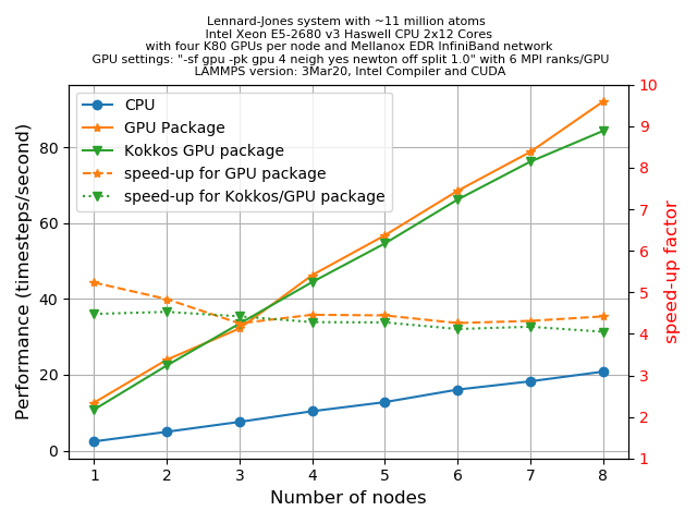
Key Points
Knowing the capabilities of your host, device and if you can use a CUDA-aware MPI runtime is required before starting a GPU run
KOKKOS compares very well with the GPU package in double precision
KOKKOS aims to be performance portable and is worth pursuing because of this
Limitations and Rules of Thumb
Overview
Teaching: 10 min
Exercises: 0 minQuestions
What are the limitations of KOKKOS and other accelerator packages?
How can I be sure that LAMMPS is working efficiently
Objectives
Identify some limitations in accelerator packages
Discussion
Nothing is perfect! Discuss amongst yourselves the limitations of different accelerator packages
Key Points
Nothing is perfect, there is no single best solution for all cases